Odtnhj

Part of a series on
Spacetime
General relativity Special relativity Doubly special relativity
Spacetime concepts Spacetime manifold Equivalence principle Lorentz transformations Minkowski space
General relativity Introduction to general relativity Mathematics of general relativity Einstein field equations
Classical gravity Introduction to gravitation Newton's law of universal gravitation
Relevant mathematics Four-vector Derivations of relativity Spacetime diagrams Differential geometry Curved spacetime Mathematics of general relativity Spacetime topology
v t e

In special relativity, a four-vector (also known as a 4-vector)^[1] is an object with four components, which transform in a specific way under Lorentz transformation. Specifically, a four-vector is an element of a four-dimensional vector space considered as a representation space of the standard representation of the Lorentz group, the (½,½) representation. It differs from a Euclidean vector in how its magnitude is determined. The transformations that preserve this magnitude are the Lorentz transformations, which include spatial rotations and boosts (a change by a constant velocity to another inertial reference frame).^[2]:ch1

Four-vectors describe, for instance, position x^μ in spacetime modeled as Minkowski space, a particle's four-momentum p^μ, the amplitude of the electromagnetic four-potential A^μ(x) at a point x in spacetime, and the elements of the subspace spanned by the gamma matrices inside the Dirac algebra.

The Lorentz group may be represented by 4×4 matrices Λ. The action of a Lorentz transformation on a general contravariant four-vector X (like the examples above), regarded as a column vector with Cartesian coordinates with respect to an inertial frame in the entries, is given by

X′=ΛX,displaystyle X^prime =Lambda X,

(matrix multiplication) where the components of the primed object refer to the new frame. Related to the examples above that are given as contravariant vectors, there are also the corresponding covariant vectors x_μ, p_μ and A_μ(x). These transform according to the rule

X′=(Λ−1)TX,displaystyle X^prime =(Lambda ^-1)^mathrm T X,

where ^T denotes the matrix transpose. This rule is different from the above rule. It corresponds to the dual representation of the standard representation. However, for the Lorentz group the dual of any representation is equivalent to the original representation. Thus the objects with covariant indices are four-vectors as well.

For an example of a well-behaved four-component object in special relativity that is not a four-vector, see bispinor. It is similarly defined, the difference being that the transformation rule under Lorentz transformations is given by a representation other than the standard representation. In this case, the rule reads X′ = Π(Λ)X, where Π(Λ) is a 4×4 matrix other than Λ. Similar remarks apply to objects with fewer or more components that are well-behaved under Lorentz transformations. These include scalars, spinors, tensors and spinor-tensors.

The article considers four-vectors in the context of special relativity. Although the concept of four-vectors also extends to general relativity, some of the results stated in this article require modification in general relativity.

Notation

The notations in this article are: lowercase bold for three-dimensional vectors, hats for three-dimensional unit vectors, capital bold for four dimensional vectors (except for the four-gradient), and tensor index notation.

Four-vector algebra

Four-vectors in a real-valued basis

A four-vector A is a vector with a "timelike" component and three "spacelike" components, and can be written in various equivalent notations:^[3]

A=(A0,A1,A2,A3)=A0E0+A1E1+A2E2+A3E3=A0E0+AiEi=AαEα=Aμdisplaystyle beginalignedmathbf A &=(A^0,,A^1,,A^2,,A^3)\&=A^0mathbf E _0+A^1mathbf E _1+A^2mathbf E _2+A^3mathbf E _3\&=A^0mathbf E _0+A^imathbf E _i\&=A^alpha mathbf E _alpha \&=A^mu endaligned

where in the last form the magnitude component and basis vector have been combined to a single element.

The upper indices indicate contravariant components. Here the standard convention is that Latin indices take values for spatial components, so that i = 1, 2, 3, and Greek indices take values for space and time components, so α = 0, 1, 2, 3, used with the summation convention. The split between the time component and the spatial components is a useful one to make when determining contractions of one four vector with other tensor quantities, such as for calculating Lorentz invariants in inner products (examples are given below), or raising and lowering indices.

In special relativity, the spacelike basis E₁, E₂, E₃ and components A¹, A², A³ are often Cartesian basis and components:

A=(At,Ax,Ay,Az)=AtEt+AxEx+AyEy+AzEzdisplaystyle beginalignedmathbf A &=(A_t,,A_x,,A_y,,A_z)\&=A_tmathbf E _t+A_xmathbf E _x+A_ymathbf E _y+A_zmathbf E _z\endaligned

although, of course, any other basis and components may be used, such as spherical polar coordinates

A=(At,Ar,Aθ,Aϕ)=AtEt+ArEr+AθEθ+AϕEϕdisplaystyle beginalignedmathbf A &=(A_t,,A_r,,A_theta ,,A_phi )\&=A_tmathbf E _t+A_rmathbf E _r+A_theta mathbf E _theta +A_phi mathbf E _phi \endaligned

or cylindrical polar coordinates,

A=(At,Ar,Aθ,Az)=AtEt+ArEr+AθEθ+AzEzdisplaystyle beginalignedmathbf A &=(A_t,,A_r,,A_theta ,,A_z)\&=A_tmathbf E _t+A_rmathbf E _r+A_theta mathbf E _theta +A_zmathbf E _z\endaligned

or any other orthogonal coordinates, or even general curvilinear coordinates. Note the coordinate labels are always subscripted as labels and are not indices taking numerical values. In general relativity, local curvilinear coordinates in a local basis must be used. Geometrically, a four-vector can still be interpreted as an arrow, but in spacetime - not just space. In relativity, the arrows are drawn as part of Minkowski diagram (also called spacetime diagram). In this article, four-vectors will be referred to simply as vectors.

It is also customary to represent the bases by column vectors:

E0=(1000),E1=(0100),E2=(0010),E3=(0001)displaystyle mathbf E _0=beginpmatrix1\0\0\0endpmatrix,,quad mathbf E _1=beginpmatrix0\1\0\0endpmatrix,,quad mathbf E _2=beginpmatrix0\0\1\0endpmatrix,,quad mathbf E _3=beginpmatrix0\0\0\1endpmatrix

so that:

A=(A0A1A2A3)displaystyle mathbf A =beginpmatrixA^0\A^1\A^2\A^3endpmatrix

The relation between the covariant and contravariant coordinates is through the Minkowski metric tensor (referred to as the metric), η which raises and lowers indices as follows:

Aμ=ημνAν,displaystyle A_mu =eta _mu nu A^nu ,,

and in various equivalent notations the covariant components are:

A=(A0,A1,A2,A3)=A0E0+A1E1+A2E2+A3E3=A0E0+AiEi=AαEαdisplaystyle beginalignedmathbf A &=(A_0,,A_1,,A_2,,A_3)\&=A_0mathbf E ^0+A_1mathbf E ^1+A_2mathbf E ^2+A_3mathbf E ^3\&=A_0mathbf E ^0+A_imathbf E ^i\&=A_alpha mathbf E ^alpha \endaligned

where the lowered index indicates it to be covariant. Often the metric is diagonal, as is the case for orthogonal coordinates (see line element), but not in general curvilinear coordinates.

The bases can be represented by row vectors:

E0=(1000),E1=(0100),E2=(0010),E3=(0001)displaystyle mathbf E ^0=beginpmatrix1&0&0&0endpmatrix,,quad mathbf E ^1=beginpmatrix0&1&0&0endpmatrix,,quad mathbf E ^2=beginpmatrix0&0&1&0endpmatrix,,quad mathbf E ^3=beginpmatrix0&0&0&1endpmatrix

so that:

A=(A0A1A2A3)displaystyle mathbf A =beginpmatrixA_0&A_1&A_2&A_3endpmatrix

The motivation for the above conventions are that the inner product is a scalar, see below for details.

Lorentz transformation

Given two inertial or rotated frames of reference, a four-vector is defined as a quantity which transforms according to the Lorentz transformation matrix Λ:

A′=ΛAdisplaystyle mathbf A '=boldsymbol Lambda mathbf A

In index notation, the contravariant and covariant components transform according to, respectively:

A′μ=ΛμνAν,A′μ=ΛμνAνdisplaystyle A'^mu =Lambda ^mu _nu A^nu ,,quad A'_mu =Lambda _mu ^nu A_nu

in which the matrix Λ has components Λ^μ_ν in row μ and column ν, and the inverse matrix Λ⁻¹ has components Λ_μ^ν in row μ and column ν.

For background on the nature of this transformation definition, see tensor. All four-vectors transform in the same way, and this can be generalized to four-dimensional relativistic tensors; see special relativity.

Pure rotations about an arbitrary axis

For two frames rotated by a fixed angle θ about an axis defined by the unit vector:

n^=(n^1,n^2,n^3),displaystyle hat mathbf n =(hat n_1,hat n_2,hat n_3),,

without any boosts, the matrix Λ has components given by:^[4]

Λ00=1displaystyle Lambda _00=1

Λ0i=Λi0=0displaystyle Lambda _0i=Lambda _i0=0

Λij=(δij−n^in^j)cos⁡θ−εijkn^ksin⁡θ+n^in^jdisplaystyle Lambda _ij=(delta _ij-hat n_ihat n_j)cos theta -varepsilon _ijkhat n_ksin theta +hat n_ihat n_j

where δ_ij is the Kronecker delta, and ε_ijk is the three-dimensional Levi-Civita symbol. The spacelike components of four-vectors are rotated, while the timelike components remain unchanged.

For the case of rotations about the z-axis only, the spacelike part of the Lorentz matrix reduces to the rotation matrix about the z-axis:

(A′0A′1A′2A′3)=(10000cos⁡θ−sin⁡θ00sin⁡θcos⁡θ00001)(A0A1A2A3) .displaystyle beginpmatrixA'^0\A'^1\A'^2\A'^3endpmatrix=beginpmatrix1&0&0&0\0&cos theta &-sin theta &0\0&sin theta &cos theta &0\0&0&0&1\endpmatrixbeginpmatrixA^0\A^1\A^2\A^3endpmatrix .

Pure boosts in an arbitrary direction

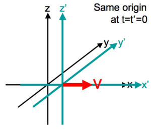
Standard configuration of coordinate systems; for a Lorentz boost in the x-direction.

For two frames moving at constant relative three-velocity v (not four-velocity, see below), it is convenient to denote and define the relative velocity in units of c by:

β=(β1,β2,β3)=1c(v1,v2,v3)=1cv.displaystyle boldsymbol beta =(beta _1,,beta _2,,beta _3)=frac 1c(v_1,,v_2,,v_3)=frac 1cmathbf v ,.

Then without rotations, the matrix Λ has components given by:^[5]

Λ00=γ,Λ0i=Λi0=−γβi,Λij=Λji=(γ−1)βiβjβ2+δij=(γ−1)vivjv2+δij,displaystyle beginalignedLambda _00&=gamma ,\Lambda _0i&=Lambda _i0=-gamma beta _i,\Lambda _ij&=Lambda _ji=(gamma -1)dfrac beta _ibeta _jbeta ^2+delta _ij=(gamma -1)dfrac v_iv_jv^2+delta _ij,\endaligned,!Lambda_0i & = "Lambda_i0 = - gamma beta_i, \"
Lambda_ij & = "Lambda_ji = ( gamma - 1 )dfracbeta_ibeta_jbeta^2 + delta_ij= ( gamma - 1 )dfracv_i v_jv^2 + delta_ij, \"
endalign
,!"/>

where the Lorentz factor is defined by:

γ=11−β⋅β,displaystyle gamma =frac 1sqrt 1-boldsymbol beta cdot boldsymbol beta ,,

and δ_ij is the Kronecker delta. Contrary to the case for pure rotations, the spacelike and timelike components are mixed together under boosts.

For the case of a boost in the x-direction only, the matrix reduces to;^[6][7]

(A′0A′1A′2A′3)=(cosh⁡ϕ−sinh⁡ϕ00−sinh⁡ϕcosh⁡ϕ0000100001)(A0A1A2A3)displaystyle beginpmatrixA'^0\A'^1\A'^2\A'^3endpmatrix=beginpmatrixcosh phi &-sinh phi &0&0\-sinh phi &cosh phi &0&0\0&0&1&0\0&0&0&1\endpmatrixbeginpmatrixA^0\A^1\A^2\A^3endpmatrixA'^0 \ A'^1 \ A'^2 \ A'^3
endpmatrix
="beginpmatrix"
coshphi &-sinhphi & 0 & 0 \
-sinhphi & coshphi & 0 & 0 \
0 & 0 & 1 & 0 \
0 & 0 & 0 & 1 \
endpmatrix
"beginpmatrix"
A^0 \ A^1 \ A^2 \ A^3
endpmatrix
"/>

Where the rapidity ϕ expression has been used, written in terms of the hyperbolic functions:

γ=cosh⁡ϕdisplaystyle gamma =cosh phi

This Lorentz matrix illustrates the boost to be a hyperbolic rotation in four dimensional spacetime, analogous to the circular rotation above in three-dimensional space.

Properties

Linearity

Four-vectors have the same linearity properties as Euclidean vectors in three dimensions. They can be added in the usual entrywise way:

A+B=(A0,A1,A2,A3)+(B0,B1,B2,B3)=(A0+B0,A1+B1,A2+B2,A3+B3)displaystyle mathbf A +mathbf B =(A^0,A^1,A^2,A^3)+(B^0,B^1,B^2,B^3)=(A^0+B^0,A^1+B^1,A^2+B^2,A^3+B^3)

and similarly scalar multiplication by a scalar λ is defined entrywise by:

λA=λ(A0,A1,A2,A3)=(λA0,λA1,λA2,λA3)displaystyle lambda mathbf A =lambda (A^0,A^1,A^2,A^3)=(lambda A^0,lambda A^1,lambda A^2,lambda A^3)

Then subtraction is the inverse operation of addition, defined entrywise by:

A+(−1)B=(A0,A1,A2,A3)+(−1)(B0,B1,B2,B3)=(A0−B0,A1−B1,A2−B2,A3−B3)displaystyle mathbf A +(-1)mathbf B =(A^0,A^1,A^2,A^3)+(-1)(B^0,B^1,B^2,B^3)=(A^0-B^0,A^1-B^1,A^2-B^2,A^3-B^3)

Minkowski tensor

Applying the Minkowski tensor η_μν to two four-vectors A and B, writing the result in dot product notation, we have, using Einstein notation:

A⋅B=AμημνBνdisplaystyle mathbf A cdot mathbf B =A^mu eta _mu nu B^nu

It is convenient to rewrite the definition in matrix form:

A⋅B=(A0A1A2A3)(η00η01η02η03η10η11η12η13η20η21η22η23η30η31η32η33)(B0B1B2B3)displaystyle mathbf Acdot B =beginpmatrixA^0&A^1&A^2&A^3endpmatrixbeginpmatrixeta _00&eta _01&eta _02&eta _03\eta _10&eta _11&eta _12&eta _13\eta _20&eta _21&eta _22&eta _23\eta _30&eta _31&eta _32&eta _33endpmatrixbeginpmatrixB^0\B^1\B^2\B^3endpmatrix

in which case η_μν above is the entry in row μ and column ν of the Minkowski metric as a square matrix. The Minkowski metric is not a Euclidean metric, because it is indefinite (see metric signature). A number of other expressions can be used because the metric tensor can raise and lower the components of A or B. For contra/co-variant components of A and co/contra-variant components of B, we have:

A⋅B=AμημνBν=AνBν=AμBμdisplaystyle mathbf A cdot mathbf B =A^mu eta _mu nu B^nu =A_nu B^nu =A^mu B_mu

so in the matrix notation:

A⋅B=(A0A1A2A3)(B0B1B2B3)=(B0B1B2B3)(A0A1A2A3)displaystyle mathbf Acdot B =beginpmatrixA_0&A_1&A_2&A_3endpmatrixbeginpmatrixB^0\B^1\B^2\B^3endpmatrix=beginpmatrixB_0&B_1&B_2&B_3endpmatrixbeginpmatrixA^0\A^1\A^2\A^3endpmatrix

while for A and B each in covariant components:

A⋅B=AμημνBνdisplaystyle mathbf A cdot mathbf B =A_mu eta ^mu nu B_nu

with a similar matrix expression to the above.

Applying the Minkowski tensor to a four-vector A with itself we get:

A⋅A=AμημνAνdisplaystyle mathbf Acdot A =A^mu eta _mu nu A^nu

which, depending on the case, may be considered the square, or its negative, of the length of the vector.

Following are two common choices for the metric tensor in the standard basis (essentially Cartesian coordinates). If orthogonal coordinates are used, there would be scale factors along the diagonal part of the spacelike part of the metric, while for general curvilinear coordinates the entire spacelike part of the metric would have components dependent on the curvilinear basis used.

Standard basis, (+−−−) signature

In the (+−−−) metric signature, evaluating the summation over indices gives:

A⋅B=A0B0−A1B1−A2B2−A3B3displaystyle mathbf A cdot mathbf B =A^0B^0-A^1B^1-A^2B^2-A^3B^3

while in matrix form:

A⋅B=(A0A1A2A3)(10000−10000−10000−1)(B0B1B2B3)displaystyle mathbf Acdot B =beginpmatrixA^0&A^1&A^2&A^3endpmatrixbeginpmatrix1&0&0&0\0&-1&0&0\0&0&-1&0\0&0&0&-1endpmatrixbeginpmatrixB^0\B^1\B^2\B^3endpmatrix

It is a recurring theme in special relativity to take the expression

A⋅B=A0B0−A1B1−A2B2−A3B3=Cdisplaystyle mathbf A cdot mathbf B =A^0B^0-A^1B^1-A^2B^2-A^3B^3=C

in one reference frame, where C is the value of the inner product in this frame, and:

A′⋅B′=A′0B′0−A′1B′1−A′2B′2−A′3B′3=C′displaystyle mathbf A 'cdot mathbf B '=A'^0B'^0-A'^1B'^1-A'^2B'^2-A'^3B'^3=C'

in another frame, in which C′ is the value of the inner product in this frame. Then since the inner product is an invariant, these must be equal:

A⋅B=A′⋅B′displaystyle mathbf A cdot mathbf B =mathbf A 'cdot mathbf B '

that is:

C=A0B0−A1B1−A2B2−A3B3=A′0B′0−A′1B′1−A′2B′2−A′3B′3displaystyle C=A^0B^0-A^1B^1-A^2B^2-A^3B^3=A'^0B'^0-A'^1B'^1-A'^2B'^2-A'^3B'^3

Considering that physical quantities in relativity are four-vectors, this equation has the appearance of a "conservation law", but there is no "conservation" involved. The primary significance of the Minkowski inner product is that for any two four-vectors, its value is invariant for all observers; a change of coordinates does not result in a change in value of the inner product. The components of the four-vectors change from one frame to another; A and A′ are connected by a Lorentz transformation, and similarly for B and B′, although the inner products are the same in all frames. Nevertheless, this type of expression is exploited in relativistic calculations on a par with conservation laws, since the magnitudes of components can be determined without explicitly performing any Lorentz transformations. A particular example is with energy and momentum in the energy-momentum relation derived from the four-momentum vector (see also below).

In this signature we have:

A⋅A=(A0)2−(A1)2−(A2)2−(A3)2displaystyle mathbf Acdot A =(A^0)^2-(A^1)^2-(A^2)^2-(A^3)^2

With the signature (+−−−), four-vectors may be classified as either spacelike if A⋅A<0displaystyle mathbf Acdot A <0, timelike if A⋅A>0displaystyle mathbf Acdot A >0, and null vectors if A⋅A=0displaystyle mathbf Acdot A =0.

Standard basis, (−+++) signature

Some authors define η with the opposite sign, in which case we have the (−+++) metric signature. Evaluating the summation with this signature:

A⋅B=−A0B0+A1B1+A2B2+A3B3displaystyle mathbf Acdot B =-A^0B^0+A^1B^1+A^2B^2+A^3B^3

while the matrix form is:

A⋅B=(A0A1A2A3)(−1000010000100001)(B0B1B2B3)displaystyle mathbf Acdot B =left(beginmatrixA^0&A^1&A^2&A^3endmatrixright)left(beginmatrix-1&0&0&0\0&1&0&0\0&0&1&0\0&0&0&1endmatrixright)left(beginmatrixB^0\B^1\B^2\B^3endmatrixright)left( beginmatrix -1 & 0 & 0 & 0 \ 0 & 1 & 0 & 0 \ 0 & 0 & 1 & 0 \ 0 & 0 & 0 & 1 endmatrix right)
left( beginmatrixB^0 \ B^1 \ B^2 \ B^3 endmatrix right) "/>

Note that in this case, in one frame:

A⋅B=−A0B0+A1B1+A2B2+A3B3=−Cdisplaystyle mathbf A cdot mathbf B =-A^0B^0+A^1B^1+A^2B^2+A^3B^3=-C

while in another:

A′⋅B′=−A′0B′0+A′1B′1+A′2B′2+A′3B′3=−C′displaystyle mathbf A 'cdot mathbf B '=-A'^0B'^0+A'^1B'^1+A'^2B'^2+A'^3B'^3=-C'

so that:

−C=−A0B0+A1B1+A2B2+A3B3=−A′0B′0+A′1B′1+A′2B′2+A′3B′3displaystyle -C=-A^0B^0+A^1B^1+A^2B^2+A^3B^3=-A'^0B'^0+A'^1B'^1+A'^2B'^2+A'^3B'^3

which is equivalent to the above expression for C in terms of A and B. Either convention will work. With the Minkowski metric defined in the two ways above, the only difference between covariant and contravariant four-vector components are signs, therefore the signs depend on which sign convention is used.

We have:

A⋅A=−(A0)2+(A1)2+(A2)2+(A3)2displaystyle mathbf Acdot A =-(A^0)^2+(A^1)^2+(A^2)^2+(A^3)^2

With the signature (−+++), four-vectors may be classified as either spacelike if A⋅A>0displaystyle mathbf Acdot A >0, timelike if A⋅A<0displaystyle mathbf Acdot A <0, and null if A⋅A=0displaystyle mathbf Acdot A =0.

Dual vectors

Applying the Minkowski tensor is often expressed as the effect of the dual vector of one vector on the other:

A⋅B=A∗(B)=AνBν.displaystyle mathbf Acdot B =A^*(mathbf B )=A_nu B^nu .

Here the A_νs are the components of the dual vector A* of A in the dual basis and called the covariant coordinates of A, while the original A^ν components are called the contravariant coordinates.

Four-vector calculus

Derivatives and differentials

In special relativity (but not general relativity), the derivative of a four-vector with respect to a scalar λ (invariant) is itself a four-vector. It is also useful to take the differential of the four-vector, dA and divide it by the differential of the scalar, dλ:

dAdifferential=dAdλderivativedλdifferentialdisplaystyle underset textdifferentialdmathbf A =underset textderivativefrac dmathbf A dlambda underset textdifferentialdlambda

where the contravariant components are:

dA=(dA0,dA1,dA2,dA3)displaystyle dmathbf A =(dA^0,dA^1,dA^2,dA^3)

while the covariant components are:

dA=(dA0,dA1,dA2,dA3)displaystyle dmathbf A =(dA_0,dA_1,dA_2,dA_3)

In relativistic mechanics, one often takes the differential of a four-vector and divides by the differential in proper time (see below).

Fundamental four-vectors

Four-position

A point in Minkowski space is a time and spatial position, called an "event", or sometimes the position four-vector or four-position or 4-position, described in some reference frame by a set of four coordinates:

R=(ct,r)displaystyle mathbf R =left(ct,mathbf r right)

where r is the three-dimensional space position vector. If r is a function of coordinate time t in the same frame, i.e. r = r(t), this corresponds to a sequence of events as t varies. The definition R⁰ = ct ensures that all the coordinates have the same units (of distance).^[8][9][10] These coordinates are the components of the position four-vector for the event.
The displacement four-vector is defined to be an "arrow" linking two events:

ΔR=(cΔt,Δr)displaystyle Delta mathbf R =left(cDelta t,Delta mathbf r right)

For the differential four-position on a world line we have, using a norm notation:

‖dR‖2=dR⋅dR=dRμdRμ=c2dτ2=ds2,displaystyle

defining the differential line element ds and differential proper time increment dτ, but this "norm" is also:

‖dR‖2=(cdt)2−dr⋅dr,displaystyle

so that:

(cdτ)2=(cdt)2−dr⋅dr.displaystyle (cdtau )^2=(cdt)^2-dmathbf r cdot dmathbf r ,.

When considering physical phenomena, differential equations arise naturally; however, when considering space and time derivatives of functions, it is unclear which reference frame these derivatives are taken with respect to. It is agreed that time derivatives are taken with respect to the proper time τdisplaystyle tau . As proper time is an invariant, this guarantees that the proper-time-derivative of any four-vector is itself a four-vector. It is then important to find a relation between this proper-time-derivative and another time derivative (using the coordinate time t of an inertial reference frame). This relation is provided by taking the above differential invariant spacetime interval, then dividing by (cdt)² to obtain:

(cdτcdt)2=1−(drcdt⋅drcdt)=1−u⋅uc2=1γ(u)2,displaystyle left(frac cdtau cdtright)^2=1-left(frac dmathbf r cdtcdot frac dmathbf r cdtright)=1-frac mathbf u cdot mathbf u c^2=frac 1gamma (mathbf u )^2,,

where u = dr/dt is the coordinate 3-velocity of an object measured in the same frame as the coordinates x, y, z, and coordinate time t, and

γ(u)=11−u⋅uc2displaystyle gamma (mathbf u )=frac 1sqrt 1-frac mathbf u cdot mathbf u c^2

is the Lorentz factor. This provides a useful relation between the differentials in coordinate time and proper time:

dt=γ(u)dτ.displaystyle dt=gamma (mathbf u )dtau ,.

This relation can also be found from the time transformation in the Lorentz transformations.

Important four-vectors in relativity theory can be defined by applying this differential ddτdisplaystyle frac ddtau .

Four-gradient

Considering that partial derivatives are linear operators, one can form a four-gradient from the partial time derivative ∂/∂t and the spatial gradient ∇. Using the standard basis, in index and abbreviated notations, the contravariant components are:

∂=(∂∂x0,−∂∂x1,−∂∂x2,−∂∂x3)=(∂0,−∂1,−∂2,−∂3)=E0∂0−E1∂1−E2∂2−E3∂3=E0∂0−Ei∂i=Eα∂α=(1c∂∂t,−∇)=(∂tc,−∇)=E01c∂∂t−∇displaystyle beginalignedboldsymbol partial &=left(frac partial partial x_0,,-frac partial partial x_1,,-frac partial partial x_2,,-frac partial partial x_3right)\&=(partial ^0,,-partial ^1,,-partial ^2,,-partial ^3)\&=mathbf E _0partial ^0-mathbf E _1partial ^1-mathbf E _2partial ^2-mathbf E _3partial ^3\&=mathbf E _0partial ^0-mathbf E _ipartial ^i\&=mathbf E _alpha partial ^alpha \&=left(frac 1cfrac partial partial t,,-nabla right)\&=left(frac partial _tc,-nabla right)\&=mathbf E _0frac 1cfrac partial partial t-nabla \endaligned

Note the basis vectors are placed in front of the components, to prevent confusion between taking the derivative of the basis vector, or simply indicating the partial derivative is a component of this four-vector. The covariant components are:

∂=(∂∂x0,∂∂x1,∂∂x2,∂∂x3)=(∂0,∂1,∂2,∂3)=E0∂0+E1∂1+E2∂2+E3∂3=E0∂0+Ei∂i=Eα∂α=(1c∂∂t,∇)=(∂tc,∇)=E01c∂∂t+∇displaystyle beginalignedboldsymbol partial &=left(frac partial partial x^0,,frac partial partial x^1,,frac partial partial x^2,,frac partial partial x^3right)\&=(partial _0,,partial _1,,partial _2,,partial _3)\&=mathbf E ^0partial _0+mathbf E ^1partial _1+mathbf E ^2partial _2+mathbf E ^3partial _3\&=mathbf E ^0partial _0+mathbf E ^ipartial _i\&=mathbf E ^alpha partial _alpha \&=left(frac 1cfrac partial partial t,,nabla right)\&=left(frac partial _tc,nabla right)\&=mathbf E ^0frac 1cfrac partial partial t+nabla \endaligned

Since this is an operator, it doesn't have a "length", but evaluating the inner product of the operator with itself gives another operator:

∂μ∂μ=1c2∂2∂t2−∇2=∂t2c2−∇2displaystyle partial ^mu partial _mu =frac 1c^2frac partial ^2partial t^2-nabla ^2=frac partial _t^2c^2-nabla ^2

called the D'Alembert operator.

Kinematics

Four-velocity

The four-velocity of a particle is defined by:

U=dXdτ=dXdtdtdτ=γ(u)(c,u),displaystyle mathbf U =frac dmathbf X dtau =frac dmathbf X dtfrac dtdtau =gamma (mathbf u )left(c,mathbf u right),

Geometrically, U is a normalized vector tangent to the world line of the particle. Using the differential of the four-position, the magnitude of the four-velocity can be obtained:

‖U‖2=UμUμ=dXμdτdXμdτ=dXμdXμdτ2=c2,mathbf U

in short, the magnitude of the four-velocity for any object is always a fixed constant:

‖U‖2=c2^2=c^2,

The norm is also:

‖U‖2=γ(u)2(c2−u⋅u),mathbf U

so that:

c2=γ(u)2(c2−u⋅u),displaystyle c^2=gamma (mathbf u )^2left(c^2-mathbf u cdot mathbf u right),,

which reduces to the definition of the Lorentz factor.

Four-acceleration

The four-acceleration is given by:

A=dUdτ=γ(u)(dγ(u)dtc,dγ(u)dtu+γ(u)a).displaystyle mathbf A =frac dmathbf U dtau =gamma (mathbf u )left(frac dgamma (mathbf u )dtc,frac dgamma (mathbf u )dtmathbf u +gamma (mathbf u )mathbf a right).

where a = du/dt is the coordinate 3-acceleration. Since the magnitude of U is a constant, the four acceleration is orthogonal to the four velocity, i.e. the Minkowski inner product of the four-acceleration and the four-velocity is zero:

A⋅U=AμUμ=dUμdτUμ=12ddτ(UμUμ)=0displaystyle mathbf A cdot mathbf U =A^mu U_mu =frac dU^mu dtau U_mu =frac 12,frac ddtau (U^mu U_mu )=0,

which is true for all world lines. The geometric meaning of four-acceleration is the curvature vector of the world line in Minkowski space.

Dynamics

Four-momentum

For a massive particle of rest mass (or invariant mass) m₀, the four-momentum is given by:

P=m0U=m0γ(u)(c,u)=(E/c,p)displaystyle mathbf P =m_0mathbf U =m_0gamma (mathbf u )(c,mathbf u )=(E/c,mathbf p )

where the total energy of the moving particle is:

E=γ(u)m0c2displaystyle E=gamma (mathbf u )m_0c^2

and the total relativistic momentum is:

p=γ(u)m0udisplaystyle mathbf p =gamma (mathbf u )m_0mathbf u

Taking the inner product of the four-momentum with itself:

‖P‖2=PμPμ=m02UμUμ=m02c2^2=P^mu P_mu =m_0^2U^mu U_mu =m_0^2c^2

and also:

‖P‖2=E2c2−p⋅pmathbf P

which leads to the energy–momentum relation:

E2=c2p⋅p+(m0c2)2.displaystyle E^2=c^2mathbf p cdot mathbf p +(m_0c^2)^2,.

This last relation is useful relativistic mechanics, essential in relativistic quantum mechanics and relativistic quantum field theory, all with applications to particle physics.

Four-force

The four-force acting on a particle is defined analogously to the 3-force as the time derivative of 3-momentum in Newton's second law:

F=dPdτ=γ(u)(1cdEdt,dpdt)=γ(u)(P/c,f)displaystyle mathbf F =frac dmathbf P dtau =gamma (mathbf u )left(frac 1cfrac dEdt,frac dmathbf p dtright)=gamma (mathbf u )(P/c,mathbf f )

where P is the power transferred to move the particle, and f is the 3-force acting on the particle. For a particle of constant invariant mass m₀, this is equivalent to

F=m0A=m0γ(u)(dγ(u)dtc,(dγ(u)dtu+γ(u)a))displaystyle mathbf F =m_0mathbf A =m_0gamma (mathbf u )left(frac dgamma (mathbf u )dtc,left(frac dgamma (mathbf u )dtmathbf u +gamma (mathbf u )mathbf a right)right)

An invariant derived from the four-force is:

F⋅U=FμUμ=m0AμUμ=0displaystyle mathbf F cdot mathbf U =F^mu U_mu =m_0A^mu U_mu =0

from the above result.

Thermodynamics

Four-heat flux

The four-heat flux vector field, is essentially similar to the 3d heat flux vector field q, in the local frame of the fluid:^[11]

Q=−k∂T=−k(1c∂T∂t,∇T)displaystyle mathbf Q =-kboldsymbol partial T=-kleft(frac 1cfrac partial Tpartial t,nabla Tright)

where T is absolute temperature and k is thermal conductivity.

Four-baryon number flux

The flux of baryons is:^[12]

S=nUdisplaystyle mathbf S =nmathbf U

where n is the number density of baryons in the local rest frame of the baryon fluid (positive values for baryons, negative for antibaryons), and U the four-velocity field (of the fluid) as above.

Four-entropy

The four-entropy vector is defined by:^[13]

s=sS+QTdisplaystyle mathbf s =smathbf S +frac mathbf Q T

where s is the entropy per baryon, and T the absolute temperature, in the local rest frame of the fluid.^[14]

Electromagnetism

Examples of four-vectors in electromagnetism include the following.

Four-current

The electromagnetic four-current (or more correctly a four-current density)^[15] is defined by

J=(ρc,j)displaystyle mathbf J =left(rho c,mathbf j right)

formed from the current density j and charge density ρ.

Four-potential

The electromagnetic four-potential (or more correctly a four-EM vector potential) defined by

A=(ϕc,a)displaystyle mathbf A =left(frac phi c,mathbf a right)

formed from the vector potential a and the scalar potential ϕ.

The four-potential is not uniquely determined, because it depends on a choice of gauge.

In the wave equation for the electromagnetic field:

(∂⋅∂)A=0displaystyle (mathbf partial cdot mathbf partial )mathbf A =0 in vacuum

(∂⋅∂)A=μ0Jdisplaystyle (mathbf partial cdot mathbf partial )mathbf A =mu _0mathbf J with a four-current source and using the Lorenz gauge condition (∂⋅A)=0displaystyle (mathbf partial cdot mathbf A )=0

Waves

Four-frequency

A photonic plane wave can be described by the four-frequency defined as

N=ν(1,n^)displaystyle mathbf N =nu left(1,hat mathbf n right)

where ν is the frequency of the wave and n^displaystyle hat mathbf n is a unit vector in the travel direction of the wave. Now:

‖N‖=NμNμ=ν2(1−n^⋅n^)=0=N^mu N_mu =nu ^2left(1-hat mathbf n cdot hat mathbf n right)=0

so the four-frequency of a photon is always a null vector.

Four-wavevector

The quantities reciprocal to time t and space r are the angular frequency ω and wave vector k, respectively. They form the components of the four-wavevector or wave four-vector:

K=(ωc,k→)=(ωc,ωvpn^).displaystyle mathbf K =left(frac omega c,vec mathbf k right)=left(frac omega c,frac omega v_pmathbf hat n right),.

A wave packet of nearly monochromatic light can be described by:

K=2πcN=2πcν(1,n^)=ωc(1,n^).displaystyle mathbf K =frac 2pi cmathbf N =frac 2pi cnu (1,hat mathbf n )=frac omega cleft(1,hat mathbf n right),.

The de Broglie relations then showed that four-wavevector applied to matter waves as well as to light waves. :

P=ℏK=(Ec,p→)=ℏ(ωc,k→).displaystyle mathbf P =hbar mathbf K =left(frac Ec,vec pright)=hbar left(frac omega c,vec kright),.

yielding E=ℏωdisplaystyle E=hbar omega and p→=ℏk→displaystyle vec p=hbar vec k, where ħ is the Planck constant divided by 2π.

The square of the norm is:

‖K‖2=KμKμ=(ωc)2−k⋅k,displaystyle

and by the de Broglie relation:

‖K‖2=1ℏ2‖P‖2=(m0cℏ)2,^2=left(frac m_0chbar right)^2,,

we have the matter wave analogue of the energy–momentum relation:

(ωc)2−k⋅k=(m0cℏ)2.displaystyle left(frac omega cright)^2-mathbf k cdot mathbf k =left(frac m_0chbar right)^2,.

Note that for massless particles, in which case m₀ = 0, we have:

(ωc)2=k⋅k,displaystyle left(frac omega cright)^2=mathbf k cdot mathbf k ,,

or ||k|| = ω/c. Note this is consistent with the above case; for photons with a 3-wavevector of modulus ω/c, in the direction of wave propagation defined by the unit vector n^displaystyle hat mathbf n .

Quantum theory

Four-probability current

In quantum mechanics, the four-probability current or probability four-current is analogous to the electromagnetic four-current:^[16]

J=(ρc,j)displaystyle mathbf J =(rho c,mathbf j )

where ρ is the probability density function corresponding to the time component, and j is the probability current vector. In non-relativistic quantum mechanics, this current is always well defined because the expressions for density and current are positive definite and can admit a probability interpretation. In relativistic quantum mechanics and quantum field theory, it is not always possible to find a current, particularly when interactions are involved.

Replacing the energy by the energy operator and the momentum by the momentum operator in the four-momentum, one obtains the four-momentum operator, used in relativistic wave equations.

Four-spin

The four-spin of a particle is defined in the rest frame of a particle to be

S=(0,s)displaystyle mathbf S =(0,mathbf s )

where s is the spin pseudovector. In quantum mechanics, not all three components of this vector are simultaneously measurable, only one component is. The timelike component is zero in the particle's rest frame, but not in any other frame. This component can be found from an appropriate Lorentz transformation.

The norm squared is the (negative of the) magnitude squared of the spin, and according to quantum mechanics we have

‖S‖2=−|s|2=−ℏ2s(s+1)mathbf s

This value is observable and quantized, with s the spin quantum number (not the magnitude of the spin vector).

Other formulations

Four-vectors in the algebra of physical space

A four-vector A can also be defined in using the Pauli matrices as a basis, again in various equivalent notations:^[17]

A=(A0,A1,A2,A3)=A0σ0+A1σ1+A2σ2+A3σ3=A0σ0+Aiσi=Aασαdisplaystyle beginalignedmathbf A &=(A^0,,A^1,,A^2,,A^3)\&=A^0boldsymbol sigma _0+A^1boldsymbol sigma _1+A^2boldsymbol sigma _2+A^3boldsymbol sigma _3\&=A^0boldsymbol sigma _0+A^iboldsymbol sigma _i\&=A^alpha boldsymbol sigma _alpha \endalignedmathbfA & = "(A^0, , A^1, , A^2, , A^3) \"
& = "A^0boldsymbolsigma_0 + A^1 boldsymbolsigma_1 + A^2 boldsymbolsigma_2 + A^3 boldsymbolsigma_3 \"
& = "A^0boldsymbolsigma_0 + A^i boldsymbolsigma_i \"
& = "A^alphaboldsymbolsigma_alpha\"
endalign"/>

or explicitly:

A=A0(1001)+A1(0110)+A2(0−ii0)+A3(100−1)=(A0+A3A1−iA2A1+iA2A0−A3)displaystyle beginalignedmathbf A &=A^0beginpmatrix1&0\0&1endpmatrix+A^1beginpmatrix0&1\1&0endpmatrix+A^2beginpmatrix0&-i\i&0endpmatrix+A^3beginpmatrix1&0\0&-1endpmatrix\&=beginpmatrixA^0+A^3&A^1-iA^2\A^1+iA^2&A^0-A^3endpmatrixendalignedmathbfA & = "A^0beginpmatrix 1 & 0 \ 0 & 1 endpmatrix + A^1 beginpmatrix 0 & 1 \ 1 & 0 endpmatrix + A^2 beginpmatrix 0 & -i \ i & 0 endpmatrix + A^3 beginpmatrix 1 & 0 \ 0 & -1 endpmatrix \"
& = "beginpmatrix A^0 + A^3 & A^1 -i A^2 \ A^1 + i A^2 & A^0 - A^3 endpmatrix"
endalign"/>

and in this formulation, the four-vector is represented as a Hermitian matrix (the matrix transpose and complex conjugate of the matrix leaves it unchanged), rather than a real-valued column or row vector. The determinant of the matrix is the modulus of the four-vector, so the determinant is an invariant:

|A|=|A0+A3A1−iA2A1+iA2A0−A3|=(A0+A3)(A0−A3)−(A1−iA2)(A1+iA2)=(A0)2−(A1)2−(A2)2−(A3)2displaystyle &=beginvmatrixA^0+A^3&A^1-iA^2\A^1+iA^2&A^0-A^3endvmatrix\&=(A^0+A^3)(A^0-A^3)-(A^1-iA^2)(A^1+iA^2)\&=(A^0)^2-(A^1)^2-(A^2)^2-(A^3)^2endaligned|mathbfA| & = "beginvmatrix A^0 + A^3 & A^1 -i A^2 \ A^1 + i A^2 & A^0 - A^3 endvmatrix \"
& = "(A^0 + A^3)(A^0 - A^3) - (A^1 -i A^2)(A^1 + i A^2) \"
& = "(A^0)^2 - (A^1)^2 - (A^2)^2 - (A^3)^2"
endalign"/>

This idea of using the Pauli matrices as basis vectors is employed in the algebra of physical space, an example of a Clifford algebra.

Four-vectors in spacetime algebra

In spacetime algebra, another example of Clifford algebra, the gamma matrices can also form a basis. (They are also called the Dirac matrices, owing to their appearance in the Dirac equation). There is more than one way to express the gamma matrices, detailed in that main article.

The Feynman slash notation is a shorthand for a four-vector A contracted with the gamma matrices:

A/=Aαγα=A0γ0+A1γ1+A2γ2+A3γ3displaystyle mathbf A !!!!/=A_alpha gamma ^alpha =A_0gamma ^0+A_1gamma ^1+A_2gamma ^2+A_3gamma ^3

The four-momentum contracted with the gamma matrices is an important case in relativistic quantum mechanics and relativistic quantum field theory. In the Dirac equation and other relativistic wave equations, terms of the form:

P/=Pαγα=P0γ0+P1γ1+P2γ2+P3γ3=Ecγ0−pxγ1−pyγ2−pzγ3displaystyle mathbf P !!!!/=P_alpha gamma ^alpha =P_0gamma ^0+P_1gamma ^1+P_2gamma ^2+P_3gamma ^3=dfrac Ecgamma ^0-p_xgamma ^1-p_ygamma ^2-p_zgamma ^3

appear, in which the energy E and momentum components (p_x, p_y, p_z) are replaced by their respective operators.

See also

• Relativistic mechanics


• paravector


• wave vector


• 
  Dust (relativity) for the number-flux four-vector


• Basic introduction to the mathematics of curved spacetime


• Minkowski space

References

• Rindler, W. Introduction to Special Relativity (2nd edn.) (1991) Clarendon Press Oxford
  ISBN 0-19-853952-5