Odtnhj

Each of the six rows is a different permutation of three distinct balls

In mathematics, the notion of permutation relates to the act of arranging all the members of a set into some sequence or order, or if the set is already ordered, rearranging (reordering) its elements, a process called permuting. These differ from combinations, which are selections of some members of a set where order is disregarded. For example, written as tuples, there are six permutations of the set 1,2,3, namely: (1,2,3), (1,3,2), (2,1,3), (2,3,1), (3,1,2), and (3,2,1). These are all the possible orderings of this three element set. As another example, an anagram of a word, all of whose letters are different, is a permutation of its letters. In this example, the letters are already ordered in the original word and the anagram is a reordering of the letters. The study of permutations of finite sets is an important topic in the fields of combinatorics and group theory. (See the articles symmetric group and permutation group for more details on the role in group theory.)

Permutations are studied in almost every branch of mathematics. They also appear in many other fields of science. In computer science they are used for analyzing sorting algorithms, in quantum physics for describing states of particles and in biology for describing RNA sequences.

The number of permutations of n distinct objects is n factorial, usually written as n!, which means the product of all positive integers less than or equal to n.

In algebra, and particularly in group theory, a permutation of a set S is defined as a bijection from S to itself.^[1][2] That is, it is a function from S to S for which every element occurs exactly once as an image value. This is related to the rearrangement of the elements of S in which each element s is replaced by the corresponding f(s). For example, the permutation (3,1,2) mentioned above is described by the function αdisplaystyle alpha defined as:

α(1)=3,α(2)=1,α(3)=2displaystyle alpha (1)=3,quad alpha (2)=1,quad alpha (3)=2.

The collection of such permutations form a group called the symmetric group of S. The key to this group's structure is the fact that the composition of two permutations (performing two given rearrangements in succession) results in another rearrangement. Permutations may act on structured objects by rearranging their components, or by certain replacements (substitutions) of symbols. Frequently the set used is S=Nn=1,2,…,ndisplaystyle S=mathbb N _n=1,2,ldots ,n, but there is no restriction on the set.

In elementary combinatorics, the k-permutations, or partial permutations, are the ordered arrangements of k distinct elements selected from a set. When k is equal to the size of the set, these are the permutations of the set.

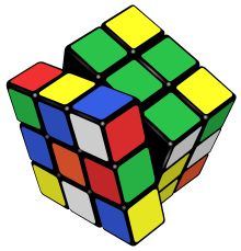
In the popular puzzle Rubik's cube invented in 1974 by Ernő Rubik, each turn of the puzzle faces creates a permutation of the surface colors.

History

The rule to determine the number of permutations of n objects was known in Indian culture at least as early as around 1150: the Lilavati by the Indian mathematician Bhaskara II contains a passage that translates to

The product of multiplication of the arithmetical series beginning and increasing by unity and continued to the number of places, will be the variations of number with specific figures.^[3]

Fabian Stedman in 1677 described factorials when explaining the number of permutations of bells in change ringing. Starting from two bells: "first, two must be admitted to be varied in two ways" which he illustrates by showing 1 2 and 2 1.^[4] He then explains that with three bells there are "three times two figures to be produced out of three" which again is illustrated. His explanation involves "cast away 3, and 1.2 will remain; cast away 2, and 1.3 will remain; cast away 1, and 2.3 will remain".^[5] He then moves on to four bells and repeats the casting away argument showing that there will be four different sets of three. Effectively this is a recursive process. He continues with five bells using the "casting away" method and tabulates the resulting 120 combinations.^[6] At this point he gives up and remarks:

Now the nature of these methods is such, that the changes on one number comprehends the changes on all lesser numbers, ... insomuch that a compleat Peal of changes on one number seemeth to be formed by uniting of the compleat Peals on all lesser numbers into one entire body;^[7]

Stedman widens the consideration of permutations; he goes on to consider the number of permutations of the letters of the alphabet and horses from a stable of 20.^[8]

A first case in which seemingly unrelated mathematical questions were studied with the help of permutations occurred around 1770, when Joseph Louis Lagrange, in the study of polynomial equations, observed that properties of the permutations of the roots of an equation are related to the possibilities to solve it. This line of work ultimately resulted, through the work of Évariste Galois, in Galois theory, which gives a complete description of what is possible and impossible with respect to solving polynomial equations (in one unknown) by radicals. In modern mathematics there are many similar situations in which understanding a problem requires studying certain permutations related to it.

Definition

In mathematics texts it is customary to denote permutations using lowercase greek letters. Commonly, either αdisplaystyle alpha and βdisplaystyle beta , or σ,τdisplaystyle sigma ,tau and πdisplaystyle pi are used.

Permutations can be defined as bijections from a set S onto itself. All permutations of a set with n elements form a symmetric group, denoted Sndisplaystyle S_n, where the group operation is function composition. Thus for two permutations, πdisplaystyle pi and σdisplaystyle sigma in the group Sndisplaystyle S_n, the four group axioms hold:

1. 
   Closure: If πdisplaystyle pi and σdisplaystyle sigma are in Sndisplaystyle S_n then so is πσ.displaystyle pi sigma .
   


2. 
   Associativity: For any three permutations π,σ,τ∈Sndisplaystyle pi ,sigma ,tau in S_n, (πσ)τ=π(στ).displaystyle (pi sigma )tau =pi (sigma tau ).
   


3. 
   Identity: There is an identity permutation, denoted iddisplaystyle mathrm id and defined by id(x)=xdisplaystyle mathrm id (x)=x for all x∈Sdisplaystyle xin S. For any σ∈Sndisplaystyle sigma in S_n, id⁡σ=σid=σ.displaystyle operatorname id sigma =sigma operatorname id =sigma .
   


4. 
   Invertibility: For every permutation π∈Sndisplaystyle pi in S_n, there exists π−1∈Sndisplaystyle pi ^-1in S_n so that ππ−1=π−1π=id.displaystyle pi pi ^-1=pi ^-1pi =operatorname id .
   

Note that in general composition of two permutations is not commutative, πσ≠σπ.displaystyle pi sigma neq sigma pi .

In this point of view it is emphasized that a permutation is a function that performs a rearrangement of a set and is not a rearrangement itself. The older and more elementary view holds that permutations are the rearrangements. Sometimes to distinguish these two views, the words active and passive forms, or in older terminology substitutions and permutations are used.^[9]

A permutation can be decomposed into one or more disjoint cycles, that is, the orbits, which are found by repeatedly tracing the application of the permutation on some elements. For example, the permutation σdisplaystyle sigma defined by σ(7)=7displaystyle sigma (7)=7 has a 1-cycle, (7)displaystyle (,7,) while the permutation πdisplaystyle pi defined by π(2)=3displaystyle pi (2)=3 and π(3)=2displaystyle pi (3)=2 has a 2-cycle (23)displaystyle (,2,3,) (for details on the syntax see the section Cycle notation below). In general, a cycle of length k, that is, consisting of k elements, is called a k-cycle.

An element in a 1-cycle (x)displaystyle (,x,) is called a fixed point of the permutation. A permutation with no fixed points is called a derangement. 2-cycles are called transpositions; such permutations merely exchange the place of two elements, leaving the others fixed.

Notations

Since writing permutations elementwise, that is, as piecewise functions, is cumbersome, several notations have been invented to represent them more compactly. Cycle notation is a popular choice for many mathematicians due to its compactness and the fact that it makes a permutation's structure transparent. It is the notation used in this article unless otherwise specified, but other notations are still widely used, especially in application areas.

Two-line notation

In Cauchy's two-line notation,^[10] one lists the elements of S in the first row, and for each one its image below it in the second row. For instance, a particular permutation of the set S = 1,2,3,4,5 can be written as:

σ=(1234525431);displaystyle sigma =beginpmatrix1&2&3&4&5\2&5&4&3&1endpmatrix;

this means that σ satisfies σ(1) = 2, σ(2) = 5, σ(3) = 4, σ(4) = 3, and σ(5) = 1. The elements of S may appear in any order in the first row. This permutation could also be written as:

σ=(3251445123).displaystyle sigma =beginpmatrix3&2&5&1&4\4&5&1&2&3endpmatrix.

One-line notation

If there is a "natural" order for the elements of S,^[a] say x1,x2,…,xndisplaystyle x_1,x_2,ldots ,x_n, then one uses this for the first row of the two-line notation:

σ=(x1x2x3⋯xnσ(x1)σ(x2)σ(x3)⋯σ(xn)).displaystyle sigma =beginpmatrixx_1&x_2&x_3&cdots &x_n\sigma (x_1)&sigma (x_2)&sigma (x_3)&cdots &sigma (x_n)endpmatrix.

Under this assumption, one may omit the first row and write the permutation in one-line notation as

(σ(x1)σ(x2)σ(x3)⋯σ(xn))displaystyle (sigma (x_1);sigma (x_2);sigma (x_3);cdots ;sigma (x_n)),

that is, an ordered arrangement of S.^[11][12] Care must be taken to distinguish one-line notation from the cycle notation described below. In mathematics literature, a common usage is to omit parentheses for one-line notation, while using them for cycle notation. The one-line notation is also called the word representation of a permutation.^[13] The example above would then be 2 5 4 3 1 since the natural order 1 2 3 4 5 would be assumed for the first row. (It is typical to use commas to separate these entries only if some have two or more digits.) This form is more compact, and is common in elementary combinatorics and computer science. It is especially useful in applications where the elements of S or the permutations are to be compared as larger or smaller.

Cycle notation

Cycle notation describes the effect of repeatedly applying the permutation on the elements of the set. It expresses the permutation as a product of cycles; since distinct cycles are disjoint, this is referred to as "decomposition into disjoint cycles".^[b]

To write down the permutation σdisplaystyle sigma in cycle notation, one proceeds as follows:

1. Write an opening bracket then select an arbitrary element x of Sdisplaystyle S and write it down: (xdisplaystyle (,x
   


2. Then trace successive applications of σdisplaystyle sigma write it down: (xσ(x)σ(σ(x))…displaystyle (,x,sigma (x),sigma (sigma (x)),ldots
   


3. Repeat until the value returns to x and write down a closing parenthesis rather than x: (xσ(x)σ(σ(x))…)displaystyle (,x,sigma (x),sigma (sigma (x)),ldots ,)
   


4. Now continue with an element y of S, not yet written down, and proceed in the same way: (xσ(x)σ(σ(x))…)(y…)displaystyle (,x,sigma (x),sigma (sigma (x)),ldots ,)(,y,ldots ,)
   


5. Repeat until all elements of S are written in cycles.

Since for every new cycle the starting point can be chosen in different ways, there are in general many different cycle notations for the same permutation; for the example above one has:

(1234525431)=(125)(34)=(34)(125)=(34)(512).displaystyle beginpmatrix1&2&3&4&5\2&5&4&3&1endpmatrix=beginpmatrix1&2&5endpmatrixbeginpmatrix3&4endpmatrix=beginpmatrix3&4endpmatrixbeginpmatrix1&2&5endpmatrix=beginpmatrix3&4endpmatrixbeginpmatrix5&1&2endpmatrix.

1-cycles are often omitted from the cycle notation, provided that the context is clear; for any element x in S not appearing in any cycle, one implicitly assumes σ(x)=xdisplaystyle sigma (x)=x.^[14] The identity permutation, which consists only of 1-cycles, can be denoted by a single 1-cycle (x), by the number 1,^[c] or by id.^[15][16]

A convenient feature of cycle notation is that one can find a permutation's inverse simply by reversing the order of the elements in the permutation's cycles. For example

[(125)(34)]−1=(521)(43)displaystyle [(,1,2,5,)(,3,4,)]^-1=(,5,2,1,)(,4,3,)

Canonical cycle notation (a.k.a. standard form)

In some combinatorial contexts it useful to fix a certain order for the elements in the cycles and of the (disjoint) cycles themselves. Miklós Bóna calls the following ordering choices the canonical cycle notation:

• in each cycle the largest element is listed first


• the cycles are sorted in increasing order of their first element

For example, (312)(54)(8)(976) is a permutation in canonical cycle notation.^[17] The canonical cycle notation does not omit one-cycles.

Richard P. Stanley calls the same choice of representation the "standard representation" of a permutation.^[18] and Martin Aigner uses the term "standard form" for the same notion.^[13] Sergey Kitaev also uses the "standard form" terminology, but reverses both choices; i.e., each cycle lists its least element first and the cycles are sorted in decreasing order of their least, that is, first elements.^[19]

Composition of permutations

There are two ways to denote the composition of two permutations. σ⋅πdisplaystyle sigma cdot pi is the function that maps any element x of the set to σ(π(x))displaystyle sigma (pi (x)). Note that the rightmost permutation is applied to the argument first,^[20]
because of the way function application is written.

Since function composition is associative, so is the composition operation on permutations: (σπ)τ=σ(πτ)displaystyle (sigma pi )tau =sigma (pi tau ). Therefore, products of more than two permutations are usually written without adding parentheses to express grouping; they are also usually written without a dot or other sign to indicate composition.

Some authors prefer the leftmost factor acting first,^[21][22][23]
but to that end permutations must be written to the right of their argument, often as an exponent, where σ acting on x is written x^σ; then the product is defined by x^σ·π = (x^σ)^π. However this gives a different rule for multiplying permutations; this article uses the definition where the rightmost permutation is applied first.

Other uses of the term permutation

The concept of a permutation as an ordered arrangement admits several generalizations that are not permutations but have been called permutations in the literature.

k-permutations of n

A weaker meaning of the term permutation, sometimes used in elementary combinatorics texts, designates those ordered arrangements in which no element occurs more than once, but without the requirement of using all the elements from a given set. These are not permutations except in special cases, but are natural generalizations of the ordered arrangement concept. Indeed, this use often involves considering arrangements of a fixed length k of elements taken from a given set of size n, in other words, these k-permutations of n are the different ordered arrangements of a k-element subset of an n-set (sometimes called variations in the older literature.^[d]) These objects are also known as partial permutations or as sequences without repetition, terms that avoid confusion with the other, more common, meaning of "permutation". The number of such kdisplaystyle k-permutations of ndisplaystyle n is denoted variously by such symbols as Pkndisplaystyle P_k^n, nPkdisplaystyle _nP_k, nPkdisplaystyle ^nP_k, Pn,kdisplaystyle P_n,k, or P(n,k)displaystyle P(n,k), and its value is given by the product^[24]

P(n,k)=n⋅(n−1)⋅(n−2)⋯(n−k+1)⏟k factorsdisplaystyle P(n,k)=underbrace ncdot (n-1)cdot (n-2)cdots (n-k+1) _k mathrm factors ,

which is 0 when k > n, and otherwise is equal to

n!(n−k)!.displaystyle frac n!(n-k)!.

The product is well defined without the assumption that ndisplaystyle n is a non-negative integer and is of importance outside combinatorics as well; it is known as the Pochhammer symbol (n)kdisplaystyle (n)_k or as the kdisplaystyle k-th falling factorial power nk_displaystyle n^underline k of ndisplaystyle n.

This usage of the term permutation is closely related to the term combination. A k-element combination of an n-set S is a k element subset of S, the elements of which are not ordered. By taking all the k element subsets of S and ordering each of them in all possible ways we obtain all the k-permutations of S. The number of k-combinations of an n-set, C(n,k), is therefore related to the number of k-permutations of n by:

C(n,k)=P(n,k)P(k,k)=n!(n−k)!k!0!=n!(n−k)!k!.displaystyle C(n,k)=frac P(n,k)P(k,k)=frac tfrac n!(n-k)!tfrac k!0!=frac n!(n-k)!,k!.

These numbers are also known as binomial coefficients and denoted (nk)displaystyle binom nk.

Permutations with repetition

Ordered arrangements of the elements of a set S of length n where repetition is allowed are called n-tuples, but have sometimes been referred to as permutations with repetition although they are not permutations in general. They are also called words over the alphabet S in some contexts. If the set S has k elements, the number of n-tuples over S is:

kn.displaystyle k^n.

There is no restriction on how often an element can appear in an n-tuple, but if restrictions are placed on how often an element can appear, this formula is no longer valid.

Permutations of multisets

Permutations of multisets

If M is a finite multiset, then a multiset permutation is an ordered arrangement of elements of M in which each element appears exactly as often as is its multiplicity in M. An anagram of a word having some repeated letters is an example of a multiset permutation.^[e] If the multiplicities of the elements of M (taken in some order) are m1displaystyle m_1, m2displaystyle m_2, …, mldisplaystyle m_l and their sum (i.e., the size of M) is n, then the number of multiset permutations of M is given by the multinomial coefficient,^[25]

(nm1,m2,…,ml)=n!m1!m2!⋯ml!=(∑i=1lmi)!∏i=1lmi!.displaystyle n choose m_1,m_2,ldots ,m_l=frac n!m_1!,m_2!,cdots ,m_l!=frac (sum _i=1^lm_i)!prod _i=1^lm_i!.

For example, the number of distinct anagrams of the word MISSISSIPPI is:^[26]

11!1!4!4!2!=34650displaystyle frac 11!1!,4!,4!,2!=34650.

A k-permutation of a multiset M is a sequence of length k of elements of M in which each element appears at most its multiplicity in M times (an element's repetition number).

Circular permutations

Permutations, when considered as arrangements, are sometimes referred to as linearly ordered arrangements. In these arrangements there is a first element, a second element, and so on. If, however, the objects are arranged in a circular manner this distinguished ordering no longer exists, that is, there is no "first element" in the arrangement, any element can be considered as the start of the arrangement. The arrangements of objects in a circular manner are called circular permutations.^[27][f] These can be formally defined as equivalence classes of ordinary permutations of the objects, for the equivalence relation generated by moving the final element of the linear arrangement to its front.

Two circular permutations are equivalent if one can be rotated into the other (that is, cycled without changing the relative positions of the elements). The following two circular permutations on four letters are considered to be the same.

 1 4
 4 3 2 1
 2 3

The circular arrangements are to be read counterclockwise, so the following two are not equivalent since no rotation can bring one to the other.

 1 1
 4 3 3 4
 2 2

The number of circular permutations of a set S with n elements is (n - 1)!.

Properties

The number of permutations of n distinct objects is n!.

The number of n-permutations with k disjoint cycles is the signless Stirling number of the first kind, denoted by c(n, k).^[28]

Permutation type

The cycles of a permutation partition the set Sndisplaystyle S_n so the lengths of the cycles of a permutation σdisplaystyle sigma forms a partition of n called the cycle type of σdisplaystyle sigma . There is a "1" in the cycle type for every fixed point of σ, a "2" for every transposition, and so on. The cycle type of β=(125)(34)(68)(7)displaystyle beta =(,1,2,5,)(,3,4,)(6,8,)(,7,) is (3,2,2,1) which is sometimes written in a more compact form as [1¹2²3¹].

The general form is [1α12α2⋯nαn]displaystyle [1^alpha _12^alpha _2dotsm n^alpha _n], where α1,…,αndisplaystyle alpha _1,ldots ,alpha _n are the number of cycles of respective length. The number of partitions of a certain type is then given by:

n!1α12α2⋯nαnα1!α2!⋯αn!displaystyle frac n!1^alpha _12^alpha _2dotsm n^alpha _nalpha _1!alpha _2!dotsm alpha _n!.

Conjugating permutations

In general, composing permutations written in cycle notation follows no easily described pattern - the cycles of the composition can be different from those being composed. However the cycle structure is preserved in the special case of conjugating a permutation σdisplaystyle sigma by another permutation πdisplaystyle pi , which means forming the product πσπ−1displaystyle pi sigma pi ^-1. Here, πσπ−1displaystyle pi sigma pi ^-1 is the conjugate of σdisplaystyle sigma and its cycle notation can be obtained by taking the cycle notation for σ and applying π to all the entries in it.^[29] It follows that two permutations are conjugate exactly when they have the same type.

Permutation order

The order of a permutation σdisplaystyle sigma is the smallest positive integer m so that σm=iddisplaystyle sigma ^m=mathrm id . It is the least common multiple of its cycles lengths. For example, the order of (132)(45)displaystyle (,1,3,2)(,4,5,) is 2⋅3=6displaystyle 2cdot 3=6.

Parity of a permutation

Every permutation of a finite set can be expressed as the product of transpositions.^[30]
Although many such expressions for a given permutation may exist, either they all contain an even or an odd number of transpositions. Thus all permutations can be classified as even or odd depending on this number.

This result can be extended so as to assign a sign, written sgnσdisplaystyle mathrm sgn sigma , to each permutation. sgnσ=+1displaystyle mathrm sgn ,sigma =+1 if σdisplaystyle sigma is positive and -1 if it is negative. Then for two permutations σdisplaystyle sigma and πdisplaystyle pi

sgn(σπ)=sgnσ⋅sgnπdisplaystyle mathrm sgn (sigma pi )=mathrm sgn ,sigma cdot mathrm sgn ,pi .

It follows that sgn(σσ−1)=+1displaystyle mathrm sgn (sigma sigma ^-1)=+1.

Matrix representation

Composition of permutations corresponds to multiplication of permutation matrices.

One can represent a permutation of 1, 2, ..., n as an n×n matrix. There are two natural ways to do so, but only one for which multiplications of matrices corresponds to multiplication of permutations in the same order: this is the one that associates to σ the matrix M whose entry M_i,j is 1 if i = σ(j), and 0 otherwise. The resulting matrix has exactly one entry 1 in each column and in each row, and is called a permutation matrix.
Here (file) is a list of these matrices for permutations of 4 elements. The Cayley table on the right shows these matrices for permutations of 3 elements.

Foata's transition lemma

There is a relationship between the one-line and the canonical cycle notation. Consider the permutation (2)(31)displaystyle (,2,)(,3,1,), in canonical cycle notation, if we erase its cycle parentheses, we obtain the permutation (2,3,1)displaystyle (2,3,1) in one-line notation. Foata's transition lemma establishes the nature of this correspondence as a bijection on the set of n-permutations (to itself).^[31] Richard P. Stanley calls this correspondence the fundamental bijection.^[18]

Let fdisplaystyle f be the parentheses-erasing transformation. The inverse of q=f(p)displaystyle q=f(p) is a bit less intuitive. Starting with the one-line notation q=q1q2⋯qndisplaystyle q=q_1q_2cdots q_n, the first cycle in canonical cycle notation must start with q1displaystyle q_1. As long as the subsequent elements are smaller than q1displaystyle q_1, we are in the same cycle. The second cycle starts at the smallest index jdisplaystyle j such that qj>q1displaystyle q_j>q_1. In other words, qjdisplaystyle q_j is larger than everything else to its left, so it is called a left-to-right maximum. Every cycle in the canonical cycle notation starts with a left-to-right maximum.^[32]

For example, in the one-line notation (3,1,2,5,4,8,9,7,6)displaystyle (3,1,2,5,4,8,9,7,6), 5 is the first element larger than 3, so the first cycle must be (312)displaystyle (,3,1,2,). Then 8 is the next element larger than 5, so the second cycle is (54)displaystyle (,5,4,). Since 9 is larger than 8, (8)displaystyle (,8,) is a cycle by itself. Finally, 9 is larger than all the remaining elements to its right, so the last cycle is (976)displaystyle (,9,7,6,).

As a first corollary, the number of n-permutations with exactly k left-to-right maxima is also equal to the signless Stirling number of the first kind, c(n,k)displaystyle c(n,k). Furthermore, Foata's mapping takes an n-permutation with k-weak excedances to an n-permutations with k − 1 ascents.^[32] For example, (2)(31) = 321 has two weak excedances (at index 1 and 2), whereas f(321) = 231 has one ascent (at index 1; i.e., from 2 to 3).

Permutations of totally ordered sets

In some applications, the elements of the set being permuted will be compared with each other. This requires that the set S has a total order so that any two elements can be compared. The set 1, 2, ..., n is totally ordered by the usual "≤" relation and so it is the most frequently used set in these applications, but in general, any totally ordered set will do. In these applications, the ordered arrangement view of a permutation is needed to talk about the positions in a permutation.

There are a number of properties that are directly related to the total ordering of S.

Ascents, descents, runs and excedances

An ascent of a permutation σ of n is any position i < n where the following value is bigger than the current one. That is, if σ = σ₁σ₂...σ_n, then i is an ascent if σ_i < σ_i+1.

For example, the permutation 3452167 has ascents (at positions) 1, 2, 5, and 6.

Similarly, a descent is a position i < n with σ_i > σ_i+1, so every i with 1≤i<ndisplaystyle 1leq i<n either is an ascent or is a descent of σ.

An ascending run of a permutation is a nonempty increasing contiguous subsequence of the permutation that cannot be extended at either end; it corresponds to a maximal sequence of successive ascents (the latter may be empty: between two successive descents there is still an ascending run of length 1). By contrast an increasing subsequence of a permutation is not necessarily contiguous: it is an increasing sequence of elements obtained from the permutation by omitting the values at some positions.
For example, the permutation 2453167 has the ascending runs 245, 3, and 167, while it has an increasing subsequence 2367.

If a permutation has k − 1 descents, then it must be the union of k ascending runs.^[33]

The number of permutations of n with k ascents is (by definition) the Eulerian number ⟨nk⟩displaystyle textstyle leftlangle n atop krightrangle ; this is also the number of permutations of n with k descents. Some authors however define the Eulerian number ⟨nk⟩displaystyle textstyle leftlangle n atop krightrangle as the number of permutations with k ascending runs, which corresponds to k − 1 descents.^[34]

An excedance of a permutation σ₁σ₂…σ_n in an index j such that σ_j > j. If the inequality is not strict (i.e., σ_j ≥ j), then j is called a weak excedance. The number of n-permutations with k excedances coincides with the number of n-permutations with k descents.^[35]

Inversions

In the 15 puzzle the goal is to get the squares in ascending order. Initial positions which have an odd number of inversions are impossible to solve.^[36]

An inversion of a permutation σ is a pair (i,j) of positions where the entries of a permutation are in the opposite order: i < j and σ_i > σ_j.^[37] So a descent is just an inversion at two adjacent positions. For example, the permutation σ = 23154 has three inversions: (1,3), (2,3), (4,5), for the pairs of entries (2,1), (3,1), (5,4).

Sometimes an inversion is defined as the pair of values (σ_i,σ_j) itself whose order is reversed; this makes no difference for the number of inversions, and this pair (reversed) is also an inversion in the above sense for the inverse permutation σ⁻¹. The number of inversions is an important measure for the degree to which the entries of a permutation are out of order; it is the same for σ and for σ⁻¹. To bring a permutation with k inversions into order (i.e., transform it into the identity permutation), by successively applying (right-multiplication by) adjacent transpositions, is always possible and requires a sequence of k such operations. Moreover, any reasonable choice for the adjacent transpositions will work: it suffices to choose at each step a transposition of i and i + 1 where i is a descent of the permutation as modified so far (so that the transposition will remove this particular descent, although it might create other descents). This is so because applying such a transposition reduces the number of inversions by 1; also note that as long as this number is not zero, the permutation is not the identity, so it has at least one descent. Bubble sort and insertion sort can be interpreted as particular instances of this procedure to put a sequence into order. Incidentally this procedure proves that any permutation σ can be written as a product of adjacent transpositions; for this one may simply reverse any sequence of such transpositions that transforms σ into the identity. In fact, by enumerating all sequences of adjacent transpositions that would transform σ into the identity, one obtains (after reversal) a complete list of all expressions of minimal length writing σ as a product of adjacent transpositions.

The number of permutations of n with k inversions is expressed by a Mahonian number,^[38] it is the coefficient of X^k in the expansion of the product

∏m=1n∑i=0m−1Xi=1(1+X)(1+X+X2)⋯(1+X+X2+⋯+Xn−1),displaystyle prod _m=1^nsum _i=0^m-1X^i=1left(1+Xright)left(1+X+X^2right)cdots left(1+X+X^2+cdots +X^n-1right),

which is also known (with q substituted for X) as the q-factorial [n]_q! . The expansion of the product appears in Necklace (combinatorics).

Permutations in computing

Numbering permutations

One way to represent permutations of n is by an integer N with 0 ≤ N < n!, provided convenient methods are given to convert between the number and the representation of a permutation as an ordered arrangement (sequence). This gives the most compact representation of arbitrary permutations, and in computing is particularly attractive when n is small enough that N can be held in a machine word; for 32-bit words this means n ≤ 12, and for 64-bit words this means n ≤ 20. The conversion can be done via the intermediate form of a sequence of numbers d_n, d_n−1, …, d₂, d₁, where d_i is a non-negative integer less than i (one may omit d₁, as it is always 0, but its presence makes the subsequent conversion to a permutation easier to describe). The first step then is to simply express N in the factorial number system, which is just a particular mixed radix representation, where for numbers up to n! the bases for successive digits are n, n − 1, …, 2, 1. The second step interprets this sequence as a Lehmer code or (almost equivalently) as an inversion table.

Rothe diagram for σ=(6,3,8,1,4,9,7,2,5)displaystyle sigma =(6,3,8,1,4,9,7,2,5)

σi i	1	2	3	4	5	6	7	8	9	Lehmer code
1	×	×	×	×	×	•				d9 = 5
2	×	×	•							d8 = 2
3	×	×		×	×		×	•		d7 = 5
4	•									d6 = 0
5		×		•						d5 = 1
6		×			×		×		•	d4 = 3
7		×			×		•			d3 = 2
8		•								d2 = 0
9					•					d1 = 0
Inversion table	3	6	1	2	4	0	2	0	0

In the Lehmer code for a permutation σ, the number d_n represents the choice made for the first term σ₁, the number d_n−1 represents the choice made for the second term
σ₂ among the remaining n − 1 elements of the set, and so forth. More precisely, each d_n+1−i gives the number of remaining elements strictly less than the term σ_i. Since those remaining elements are bound to turn up as some later term σ_j, the digit d_n+1−i counts the inversions (i,j) involving i as smaller index (the number of values j for which i < j and σ_i > σ_j). The inversion table for σ is quite similar, but here d_n+1−k counts the number of inversions (i,j) where k = σ_j occurs as the smaller of the two values appearing in inverted order.^[39] Both encodings can be visualized by an n by n Rothe diagram^[40] (named after Heinrich August Rothe) in which dots at (i,σ_i) mark the entries of the permutation, and a cross at (i,σ_j) marks the inversion (i,j); by the definition of inversions a cross appears in any square that comes both before the dot (j,σ_j) in its column, and before the dot (i,σ_i) in its row. The Lehmer code lists the numbers of crosses in successive rows, while the inversion table lists the numbers of crosses in successive columns; it is just the Lehmer code for the inverse permutation, and vice versa.

To effectively convert a Lehmer code d_n, d_n−1, ..., d₂, d₁ into a permutation of an ordered set S, one can start with a list of the elements of S in increasing order, and for i increasing from 1 to n set σ_i to the element in the list that is preceded by d_n+1−i other ones, and remove that element from the list. To convert an inversion table d_n, d_n−1, ..., d₂, d₁ into the corresponding permutation, one can traverse the numbers from d₁ to d_n while inserting the elements of S from largest to smallest into an initially empty sequence; at the step using the number d from the inversion table, the element from S inserted into the sequence at the point where it is preceded by d elements already present. Alternatively one could process the numbers from the inversion table and the elements of S both in the opposite order, starting with a row of n empty slots, and at each step place the element from S into the empty slot that is preceded by d other empty slots.

Converting successive natural numbers to the factorial number system produces those sequences in lexicographic order (as is the case with any mixed radix number system), and further converting them to permutations preserves the lexicographic ordering, provided the Lehmer code interpretation is used (using inversion tables, one gets a different ordering, where one starts by comparing permutations by the place of their entries 1 rather than by the value of their first entries). The sum of the numbers in the factorial number system representation gives the number of inversions of the permutation, and the parity of that sum gives the signature of the permutation. Moreover, the positions of the zeroes in the inversion table give the values of left-to-right maxima of the permutation (in the example 6, 8, 9) while the positions of the zeroes in the Lehmer code are the positions of the right-to-left minima (in the example positions the 4, 8, 9 of the values 1, 2, 5); this allows computing the distribution of such extrema among all permutations. A permutation with Lehmer code d_n, d_n−1, ..., d₂, d₁ has an ascent n − i if and only if d_i ≥ d_i+1.

Algorithms to generate permutations

In computing it may be required to generate permutations of a given sequence of values. The methods best adapted to do this depend on whether one wants some randomly chosen permutations, or all permutations, and in the latter case if a specific ordering is required. Another question is whether possible equality among entries in the given sequence is to be taken into account; if so, one should only generate distinct multiset permutations of the sequence.

An obvious way to generate permutations of n is to generate values for the Lehmer code (possibly using the factorial number system representation of integers up to n!), and convert those into the corresponding permutations. However, the latter step, while straightforward, is hard to implement efficiently, because it requires n operations each of selection from a sequence and deletion from it, at an arbitrary position; of the obvious representations of the sequence as an array or a linked list, both require (for different reasons) about n²/4 operations to perform the conversion. With n likely to be rather small (especially if generation of all permutations is needed) that is not too much of a problem, but it turns out that both for random and for systematic generation there are simple alternatives that do considerably better. For this reason it does not seem useful, although certainly possible, to employ a special data structure that would allow performing the conversion from Lehmer code to permutation in O(n log n) time.

Random generation of permutations

For generating random permutations of a given sequence of n values, it makes no difference whether one applies a randomly selected permutation of n to the sequence, or chooses a random element from the set of distinct (multiset) permutations of the sequence. This is because, even though in case of repeated values there can be many distinct permutations of n that result in the same permuted sequence, the number of such permutations is the same for each possible result. Unlike for systematic generation, which becomes unfeasible for large n due to the growth of the number n!, there is no reason to assume that n will be small for random generation.

The basic idea to generate a random permutation is to generate at random one of the n! sequences of integers d₁,d₂,...,d_n satisfying 0 ≤ d_i < i (since d₁ is always zero it may be omitted) and to convert it to a permutation through a bijective correspondence. For the latter correspondence one could interpret the (reverse) sequence as a Lehmer code, and this gives a generation method first published in 1938 by Ronald Fisher and Frank Yates.^[41]
While at the time computer implementation was not an issue, this method suffers from the difficulty sketched above to convert from Lehmer code to permutation efficiently. This can be remedied by using a different bijective correspondence: after using d_i to select an element among i remaining elements of the sequence (for decreasing values of i), rather than removing the element and compacting the sequence by shifting down further elements one place, one swaps the element with the final remaining element. Thus the elements remaining for selection form a consecutive range at each point in time, even though they may not occur in the same order as they did in the original sequence. The mapping from sequence of integers to permutations is somewhat complicated, but it can be seen to produce each permutation in exactly one way, by an immediate induction. When the selected element happens to be the final remaining element, the swap operation can be omitted. This does not occur sufficiently often to warrant testing for the condition, but the final element must be included among the candidates of the selection, to guarantee that all permutations can be generated.

The resulting algorithm for generating a random permutation of a[0], a[1], ..., a[n − 1] can be described as follows in pseudocode:

 for i from n downto 2
 do   di ← random element of 0, ..., i − 1 
 swap a[di] and a[i − 1]

This can be combined with the initialization of the array a[i] = i as follows

 for i from 0 to n−1
 do   di+1 ← random element of 0, ..., i 
 a[i] ← a[di+1]
 a[di+1] ← i

If d_i+1 = i, the first assignment will copy an uninitialized value, but the second will overwrite it with the correct value i.

However, Fisher-Yates is not the fastest algorithm for generating a permutation, because Fisher-Yates is essentially a sequential algorithm and "divide and conquer" procedures can achieve the same result in parallel.^[42]

Generation in lexicographic order

There are many ways to systematically generate all permutations of a given sequence.^[43]
One classical algorithm, which is both simple and flexible, is based on finding the next permutation in lexicographic ordering, if it exists. It can handle repeated values, for which case it generates the distinct multiset permutations each once. Even for ordinary permutations it is significantly more efficient than generating values for the Lehmer code in lexicographic order (possibly using the factorial number system) and converting those to permutations. To use it, one starts by sorting the sequence in (weakly) increasing order (which gives its lexicographically minimal permutation), and then repeats advancing to the next permutation as long as one is found. The method goes back to Narayana Pandita in 14th century India, and has been frequently rediscovered ever since.^[44]

The following algorithm generates the next permutation lexicographically after a given permutation. It changes the given permutation in-place.

1. Find the largest index k such that a[k] < a[k + 1]. If no such index exists, the permutation is the last permutation.


2. Find the largest index l greater than k such that a[k] < a[l].


3. Swap the value of a[k] with that of a[l].


4. Reverse the sequence from a[k + 1] up to and including the final element a[n].

For example, given the sequence [1, 2, 3, 4] (which is in increasing order), and given that the index is zero-based, the steps are as follows:

1. Index k = 2, because 3 is placed at an index that satisfies condition of being the largest index that is still less than a[k + 1] which is 4.


2. Index l = 3, because 4 is the only value in the sequence that is greater than 3 in order to satisfy the condition a[k] < a[l].


3. The values of a[2] and a[3] are swapped to form the new sequence [1,2,4,3].


4. The sequence after k-index a[2] to the final element is reversed. Because only one value lies after this index (the 3), the sequence remains unchanged in this instance. Thus the lexicographic successor of the initial state is permuted: [1,2,4,3].

Following this algorithm, the next lexicographic permutation will be [1,3,2,4], and the 24th permutation will be [4,3,2,1] at which point a[k] < a[k + 1] does not exist, indicating that this is the last permutation.

This method uses about 3 comparisons and 1.5 swaps per permutation, amortized over the whole sequence, not counting the initial sort.^[45]

Generation with minimal changes

An alternative to the above algorithm, the Steinhaus–Johnson–Trotter algorithm, generates an ordering on all the permutations of a given sequence with the property that any two consecutive permutations in its output differ by swapping two adjacent values. This ordering on the permutations was known to 17th-century English bell ringers, among whom it was known as "plain changes". One advantage of this method is that the small amount of change from one permutation to the next allows the method to be implemented in constant time per permutation. The same can also easily generate the subset of even permutations, again in constant time per permutation, by skipping every other output permutation.^[44]

An alternative to Steinhaus–Johnson–Trotter is Heap's algorithm,^[46] said by Robert Sedgewick in 1977 to be the fastest algorithm of generating permutations in applications.^[43]

Meandric permutations

Meandric systems give rise to meandric permutations, a special subset of alternate permutations. An alternate permutation of the set 1, 2, …, 2n is a cyclic permutation (with no fixed points) such that the digits in the cyclic notation form alternate between odd and even integers. Meandric permutations are useful in the analysis of RNA secondary structure. Not all alternate permutations are meandric. A modification of Heap's algorithm has been used to generate all alternate permutations of order n (that is, of length 2n) without generating all (2n)! permutations.^{[47][unreliable source?]} Generation of these alternate permutations is needed before they are analyzed to determine if they are meandric or not.

The algorithm is recursive. The following table exhibits a step in the procedure. In the previous step, all alternate permutations of length 5 have been generated. Three copies of each of these have a "6" added to the right end, and then a different transposition involving this last entry and a previous entry in an even position is applied (including the identity; i.e., no transposition).

Applications

Permutations are used in the interleaver component of the error detection and correction algorithms, such as turbo codes, for example 3GPP Long Term Evolution mobile telecommunication standard uses these ideas (see 3GPP technical specification 36.212 ^[48]).
Such applications raise the question of fast generation of permutations satisfying certain desirable properties. One of the methods is based on the permutation polynomials. Also as a base for optimal hashing in Unique Permutation Hashing.^[49]

See also

Notes

References

Bibliography

• 
  Bogart, Kenneth P. (1990), Introductory Combinatorics (2nd ed.), Harcourt Brace Jovanovich, ISBN 0-15-541576-X
  


• 
  Bóna, Miklós (2004), Combinatorics of Permutations, Chapman Hall-CRC, ISBN 1-58488-434-7
  


• 
  Bona, Miklos (2012), Combinatorics of Permutations (2nd ed.), CRC Press, ISBN 978-1-4398-5051-0
  


• 
  Brualdi, Richard A. (2010), Introductory Combinatorics (5th ed.), Prentice-Hall, ISBN 978-0-13-602040-0
  


• 
  Cameron, Peter J. (1994), Combinatorics: Topics, Techniques, Algorithms, Cambridge University Press, ISBN 0-521-45761-0
  


• 
  Carmichael, Robert D. (1956) [1937], Introduction to the theory of Groups of Finite Order, Dover, ISBN 0-486-60300-8
  


• 
  Gerstein, Larry J. (1987), Discrete Mathematics and Algebraic Structures, W.H. Freeman and Co., ISBN 0-7167-1804-9
  


• 
  Hall, Marshall, Jr. (1959), The Theory of Groups, MacMillan
  


• 
  Humphreys, J. F. (1996), A course in group theory, Oxford University Press, ISBN 978-0-19-853459-4
  


• 
  Knuth, Donald (1973), Sorting and Searching, The Art of Computer Programming, 3 This book mentions the Lehmer code (without using that name) as a variant C₁,...,C_n of inversion tables in exercise 5.1.1−7 (p. 19), together with two other variants.


• 
  Knuth, Donald (2005), Generating All Tuples and Permutations, The Art of Computer Programming, 4, Addison–Wesley, ISBN 0-201-85393-0 Fascicle 2, first printing.


• 
  McCoy, Neal H. (1968), Introduction To Modern Algebra, Revised Edition, Boston: Allyn and Bacon, LCCN 68015225
  


• 
  Nering, Evar D. (1970), Linear Algebra and Matrix Theory (2nd ed.), New York: Wiley, LCCN 76091646
  


• 
  Rotman, Joseph J. (2002), Advanced Modern Algebra, Prentice-Hall, ISBN 0-13-087868-5
  


• 
  Stedman, Fabian (1677), Campanalogia, London The publisher is given as "W.S." who may have been William Smith, possibly acting as agent for the Society of College Youths, to which society the "Dedicatory" is addressed. In quotations the original long "S" has been replaced by a modern short "s".
  

Further reading

• 
  Biggs, Norman L. (2002), Discrete Mathematics (2nd ed.), Oxford University Press, ISBN 0-19-850717-8
  


• 
  Foata, Dominique; Schutzenberger, Marcel-Paul (1970), Théorie Géométrique des Polynômes Eulériens, Lecture Notes in Mathematics, 138, Berlin, Heidelberg: Springer-Verlag, ISBN 978-3-540-04927-2. The link is to a freely available retyped (LaTeX'ed) and revised version of the text originally published by Springer-Verlag.


• 
  Knuth, Donald (1998), Sorting and Searching, The Art of Computer Programming, 3 (Second ed.), Addison–Wesley, ISBN 0-201-89685-0. Section 5.1: Combinatorial Properties of Permutations, pp. 11–72.

External links

• 
  Hazewinkel, Michiel, ed. (2001) [1994], "Permutation", Encyclopedia of Mathematics, Springer Science+Business Media B.V. / Kluwer Academic Publishers, ISBN 978-1-55608-010-4
  

Wikiversity has learning resources about Permutation notation

Wikimedia Commons has media related to Permutations.

References

^ McCoy (1968, p. 152)
^ Nering (1970, p. 86)
^ Biggs, N. L. (1979). "The Roots of Combinatorics". Historia Math. 6 (2): 109–136. doi:10.1016/0315-0860(79)90074-0..mw-parser-output cite.citationfont-style:inherit.mw-parser-output qquotes:"""""""'""'".mw-parser-output code.cs1-codecolor:inherit;background:inherit;border:inherit;padding:inherit.mw-parser-output .cs1-lock-free abackground:url("//upload.wikimedia.org/wikipedia/commons/thumb/6/65/Lock-green.svg/9px-Lock-green.svg.png")no-repeat;background-position:right .1em center.mw-parser-output .cs1-lock-limited a,.mw-parser-output .cs1-lock-registration abackground:url("//upload.wikimedia.org/wikipedia/commons/thumb/d/d6/Lock-gray-alt-2.svg/9px-Lock-gray-alt-2.svg.png")no-repeat;background-position:right .1em center.mw-parser-output .cs1-lock-subscription abackground:url("//upload.wikimedia.org/wikipedia/commons/thumb/a/aa/Lock-red-alt-2.svg/9px-Lock-red-alt-2.svg.png")no-repeat;background-position:right .1em center.mw-parser-output .cs1-subscription,.mw-parser-output .cs1-registrationcolor:#555.mw-parser-output .cs1-subscription span,.mw-parser-output .cs1-registration spanborder-bottom:1px dotted;cursor:help.mw-parser-output .cs1-hidden-errordisplay:none;font-size:100%.mw-parser-output .cs1-visible-errorfont-size:100%.mw-parser-output .cs1-subscription,.mw-parser-output .cs1-registration,.mw-parser-output .cs1-formatfont-size:95%.mw-parser-output .cs1-kern-left,.mw-parser-output .cs1-kern-wl-leftpadding-left:0.2em.mw-parser-output .cs1-kern-right,.mw-parser-output .cs1-kern-wl-rightpadding-right:0.2em
^ Stedman 1677, p. 4.
^ Stedman 1677, p. 5.
^ Stedman 1677, pp. 6—7.
^ Stedman 1677, p. 8.
^ Stedman 1677, pp. 13—18.
^ Cameron 1994, p. 29, footnote 3.
^ Wussing, Hans (2007), The Genesis of the Abstract Group Concept: A Contribution to the History of the Origin of Abstract Group Theory, Courier Dover Publications, p. 94, ISBN 9780486458687,Cauchy used his permutation notation—in which the arrangements are written one below the other and both are enclosed in parentheses—for the first time in 1815.
^ Bogart 1990, p. 17
^ Gerstein 1987, p. 217
^ ab Aigner, Martin (2007). A Course in Enumeration. Springer GTM 238. pp. 24–25. ISBN 978-3-540-39035-0.
^ Hall 1959, p. 54
^ Rotman 2002, p. 41
^ Bogart 1990, p. 487
^ Bona 2012, p.87 [Note that the book has a typo/error here, as it gives (45) instead of (54).]
^ ab Stanley, Richard P. (2012). Enumerative Combinatorics: Volume I, Second Edition. Cambridge University Press. p. 23. ISBN 978-1-107-01542-5.
^ Kitaev, Sergey (2011). Patterns in Permutations and Words. Springer Science & Business Media. p. 119. ISBN 978-3-642-17333-2.
^
Biggs, Norman L.; White, A. T. (1979). Permutation groups and combinatorial structures. Cambridge University Press. ISBN 0-521-22287-7.
Dixon, John D.; Mortimer, Brian (1996). Permutation Groups. Springer. ISBN 0-387-94599-7.
Cameron, Peter J. (1999). Permutation groups. Cambridge University Press. ISBN 0-521-65302-9.
Jerrum, M. (1986). "A compact representation of permutation groups". J. Algorithms. 7 (1): 60–78. doi:10.1016/0196-6774(86)90038-6.
^ Charalambides, Ch A. (2002). Enumerative Combinatorics. CRC Press. p. 42. ISBN 978-1-58488-290-9.
^ Brualdi 2010, p. 46, Theorem 2.4.2
^ Brualdi 2010, p. 47
^ Brualdi 2010, p. 39
^ Bona 2012, pp. 97–103.
^ Humphreys 1996, p. 84.
^ Hall 1959, p. 60
^ Bona 2012, pp. 109-110.
^ ab Bona 2012, pp. 109–110.
^ Bóna 2004, p. 4f.
^ Bona 2012, pp. 4–5.
^ Bona 2012, p. 25.
^ Slocum, Jerry; Weisstein, Eric W. (1999). "15 - puzzle". MathWorld. Wolfram Research, Inc. Retrieved October 4, 2014.
^ Bóna 2004, p. 43.
^ Bóna 2004, pp. 43ff.
^ Knuth 1973, p. 12.
^ H. A. Rothe, Sammlung combinatorisch-analytischer Abhandlungen 2 (Leipzig, 1800), 263−305. Cited in Knuth 1973, p. 14
^ Fisher, R.A.; Yates, F. (1948) [1938]. Statistical tables for biological, agricultural and medical research (3rd ed.). London: Oliver & Boyd. pp. 26–27. OCLC 14222135.
^ Bacher, A.; Bodini, O.; Hwang, H.K.; Tsai, T.H. (2017). "Generating Random Permutations by Coin Tossing: Classical Algorithms, New Analysis, and Modern Implementation" (ACM Trans. Algorithms 13(2): 24:1-24:43 ed.). pp. 24–43.
^ ab Sedgewick, R (1977). "Permutation generation methods" (PDF). Computing Surveys. 9 (2): 137–164. doi:10.1145/356689.356692.
^ ab Knuth 2005, pp. 1–26.
^ "std::next_permutation". cppreference.com. 4 December 2017. Retrieved 31 March 2018.
^ Heap, B. R. (1963). "Permutations by Interchanges" (PDF). The Computer Journal. 6 (3): 293–4. doi:10.1093/comjnl/6.3.293.
Alexiou, A.; Psiha, M.; Vlamos, P. (2011). "Combinatorial permutation based algorithm for representation of closed RNA secondary structures". Bioinformation. 7 (2): 91–95. doi:10.6026/97320630007091. PMC 3174042. PMID 21938211.
^ 3GPP TS 36.212
^ Dolev, Shlomi; Lahiani, Limor; Haviv, Yinnon (2013). "Unique permutation hashing". Theoretical Computer Science. 475: 59–65. doi:10.1016/j.tcs.2012.12.047.