Deformation (mechanics)

The deformation of a thin straight rod into a closed loop. The length of the rod remains almost unchanged during the deformation, which indicates that the strain is small. In this particular case of bending, displacements associated with rigid translations and rotations of material elements in the rod are much greater than displacements associated with straining.
| Continuum mechanics | |||||||
|---|---|---|---|---|---|---|---|
Laws
| |||||||
Solid mechanics
| |||||||
Fluid mechanics
| |||||||
Rheology
| |||||||
Scientists
| |||||||
Deformation in continuum mechanics is the transformation of a body from a reference configuration to a current configuration.[1] A configuration is a set containing the positions of all particles of the body.
A deformation may be caused by external loads,[2]body forces (such as gravity or electromagnetic forces), or changes in temperature, moisture content, or chemical reactions, etc.
Strain is a description of deformation in terms of relative displacement of particles in the body that excludes rigid-body motions. Different equivalent choices may be made for the expression of a strain field depending on whether it is defined with respect to the initial or the final configuration of the body and on whether the metric tensor or its dual is considered.
In a continuous body, a deformation field results from a stress field induced by applied forces or is due to changes in the temperature field inside the body. The relation between stresses and induced strains is expressed by constitutive equations, e.g., Hooke's law for linear elastic materials. Deformations which are recovered after the stress field has been removed are called elastic deformations. In this case, the continuum completely recovers its original configuration. On the other hand, irreversible deformations remain even after stresses have been removed. One type of irreversible deformation is plastic deformation, which occurs in material bodies after stresses have attained a certain threshold value known as the elastic limit or yield stress, and are the result of slip, or dislocation mechanisms at the atomic level. Another type of irreversible deformation is viscous deformation, which is the irreversible part of viscoelastic deformation.
In the case of elastic deformations, the response function linking strain to the deforming stress is the compliance tensor of the material.
Contents
1 Strain
1.1 Strain measures
1.1.1 Engineering strain
1.1.2 Stretch ratio
1.1.3 True strain
1.1.4 Green strain
1.1.5 Almansi strain
1.2 Normal and shear strain
1.2.1 Normal strain
1.2.2 Shear strain
1.3 Metric tensor
2 Description of deformation
2.1 Affine deformation
2.2 Rigid body motion
3 Displacement
3.1 Displacement gradient tensor
4 Examples of deformations
4.1 Plane deformation
4.1.1 Isochoric plane deformation
4.1.2 Simple shear
5 See also
6 References
7 Further reading
Strain
Strain is a measure of deformation representing the displacement between particles in the body relative to a reference length.
A general deformation of a body can be expressed in the form x = F(X) where X is the reference position of material points in the body. Such a measure does not distinguish between rigid body motions (translations and rotations) and changes in shape (and size) of the body. A deformation has units of length.
We could, for example, define strain to be
- ε≐∂∂X(x−X)=F′−I,displaystyle boldsymbol varepsilon doteq cfrac partial partial mathbf X left(mathbf x -mathbf X right)=boldsymbol F'-boldsymbol I,

where I is the identity tensor.
Hence strains are dimensionless and are usually expressed as a decimal fraction, a percentage or in parts-per notation. Strains measure how much a given deformation differs locally from a rigid-body deformation.[3]
A strain is in general a tensor quantity. Physical insight into strains can be gained by observing that a given strain can be decomposed into normal and shear components. The amount of stretch or compression along material line elements or fibers is the normal strain, and the amount of distortion associated with the sliding of plane layers over each other is the shear strain, within a deforming body.[4] This could be applied by elongation, shortening, or volume changes, or angular distortion.[5]
The state of strain at a material point of a continuum body is defined as the totality of all the changes in length of material lines or fibers, the normal strain, which pass through that point and also the totality of all the changes in the angle between pairs of lines initially perpendicular to each other, the shear strain, radiating from this point. However, it is sufficient to know the normal and shear components of strain on a set of three mutually perpendicular directions.
If there is an increase in length of the material line, the normal strain is called tensile strain, otherwise, if there is reduction or compression in the length of the material line, it is called compressive strain.
Strain measures
Depending on the amount of strain, or local deformation, the analysis of deformation is subdivided into three deformation theories:
Finite strain theory, also called large strain theory, large deformation theory, deals with deformations in which both rotations and strains are arbitrarily large. In this case, the undeformed and deformed configurations of the continuum are significantly different and a clear distinction has to be made between them. This is commonly the case with elastomers, plastically-deforming materials and other fluids and biological soft tissue.
Infinitesimal strain theory, also called small strain theory, small deformation theory, small displacement theory, or small displacement-gradient theory where strains and rotations are both small. In this case, the undeformed and deformed configurations of the body can be assumed identical. The infinitesimal strain theory is used in the analysis of deformations of materials exhibiting elastic behavior, such as materials found in mechanical and civil engineering applications, e.g. concrete and steel.
Large-displacement or large-rotation theory, which assumes small strains but large rotations and displacements.
In each of these theories the strain is then defined differently. The engineering strain is the most common definition applied to materials used in mechanical and structural engineering, which are subjected to very small deformations. On the other hand, for some materials, e.g. elastomers and polymers, subjected to large deformations, the engineering definition of strain is not applicable, e.g. typical engineering strains greater than 1%,[6] thus other more complex definitions of strain are required, such as stretch, logarithmic strain, Green strain, and Almansi strain.
Engineering strain
The Cauchy strain or engineering strain is expressed as the ratio of total deformation to the initial dimension of the material body in which the forces are being applied. The engineering normal strain or engineering extensional strain or nominal strain e of a material line element or fiber axially loaded is expressed as the change in length ΔL per unit of the original length L of the line element or fibers. The normal strain is positive if the material fibers are stretched and negative if they are compressed. Thus, we have
- e=ΔLL=l−LLdisplaystyle e=frac Delta LL=frac l-LL

where e is the engineering normal strain, L is the original length of the fiber and l is the final length of the fiber. Measures of strain are often expressed in parts per million or microstrains.
The true shear strain is defined as the change in the angle (in radians) between two material line elements initially perpendicular to each other in the undeformed or initial configuration. The engineering shear strain is defined as the tangent of that angle, and is equal to the length of deformation at its maximum divided by the perpendicular length in the plane of force application which sometimes makes it easier to calculate.
Stretch ratio
The stretch ratio or extension ratio is a measure of the extensional or normal strain of a differential line element, which can be defined at either the undeformed configuration or the deformed configuration. It is defined as the ratio between the final length l and the initial length L of the material line.
- λ=lLdisplaystyle lambda =frac lL

The extension ratio is approximately related to the engineering strain by
- e=l−LL=λ−1displaystyle e=frac l-LL=lambda -1

This equation implies that the normal strain is zero, so that there is no deformation when the stretch is equal to unity.
The stretch ratio is used in the analysis of materials that exhibit large deformations, such as elastomers, which can sustain stretch ratios of 3 or 4 before they fail. On the other hand, traditional engineering materials, such as concrete or steel, fail at much lower stretch ratios.
True strain
The logarithmic strain ε, also called, true strain or Hencky strain [7]. Considering an incremental strain (Ludwik)
- δε=δlldisplaystyle delta varepsilon =frac delta ll

the logarithmic strain is obtained by integrating this incremental strain:
- ∫δε=∫Llδllε=ln(lL)=ln(λ)=ln(1+e)=e−e22+e33−⋯displaystyle beginalignedint delta varepsilon &=int _L^lfrac delta ll\varepsilon &=ln left(frac lLright)=ln(lambda )\&=ln(1+e)\&=e-frac e^22+frac e^33-cdots \endaligned

where e is the engineering strain. The logarithmic strain provides the correct measure of the final strain when deformation takes place in a series of increments, taking into account the influence of the strain path.[4]
Green strain
The Green strain is defined as:
- εG=12(l2−L2L2)=12(λ2−1)displaystyle varepsilon _G=tfrac 12left(frac l^2-L^2L^2right)=tfrac 12(lambda ^2-1)

Almansi strain
The Euler-Almansi strain is defined as
- εE=12(l2−L2l2)=12(1−1λ2)displaystyle varepsilon _E=tfrac 12left(frac l^2-L^2l^2right)=tfrac 12left(1-frac 1lambda ^2right)

Normal and shear strain

Two-dimensional geometric deformation of an infinitesimal material element.
Strains are classified as either normal or shear. A normal strain is perpendicular to the face of an element, and a shear strain is parallel to it. These definitions are consistent with those of normal stress and shear stress.
Normal strain
For an isotropic material that obeys Hooke's law, a normal stress will cause a normal strain. Normal strains produce dilations.
Consider a two-dimensional, infinitesimal, rectangular material element with dimensions dx × dy, which, after deformation, takes the form of a rhombus. From the geometry of the adjacent figure we have
- length(AB)=dxdisplaystyle mathrm length (AB)=dx,

and
- length(ab)=(dx+∂ux∂xdx)2+(∂uy∂xdx)2=dx 1+2∂ux∂x+(∂ux∂x)2+(∂uy∂x)2displaystyle beginalignedmathrm length (ab)&=sqrt left(dx+frac partial u_xpartial xdxright)^2+left(frac partial u_ypartial xdxright)^2\&=dx~sqrt 1+2frac partial u_xpartial x+left(frac partial u_xpartial xright)^2+left(frac partial u_ypartial xright)^2\endaligned,!

For very small displacement gradients the squares of the derivatives are negligible and we have
- length(ab)≈dx+∂ux∂xdxdisplaystyle mathrm length (ab)approx dx+frac partial u_xpartial xdx

The normal strain in the x-direction of the rectangular element is defined by
- εx=extensionoriginal length=length(ab)−length(AB)length(AB)=∂ux∂xdisplaystyle varepsilon _x=frac textextensiontextoriginal length=frac mathrm length (ab)-mathrm length (AB)mathrm length (AB)=frac partial u_xpartial x

Similarly, the normal strain in the y- and z-directions becomes
- εy=∂uy∂y,εz=∂uz∂zdisplaystyle varepsilon _y=frac partial u_ypartial yquad ,qquad varepsilon _z=frac partial u_zpartial z,!

Shear strain
| Shear strain | |
|---|---|
Common symbols | γ or ε |
| SI unit | 1, or radian |
Derivations from other quantities | γ = τ/G |
The engineering shear strain (γxy) is defined as the change in angle between lines AC and AB. Therefore,
- γxy=α+βdisplaystyle gamma _xy=alpha +beta ,!

From the geometry of the figure, we have
- tanα=∂uy∂xdxdx+∂ux∂xdx=∂uy∂x1+∂ux∂xtanβ=∂ux∂ydydy+∂uy∂ydy=∂ux∂y1+∂uy∂ydisplaystyle beginalignedtan alpha &=frac tfrac partial u_ypartial xdxdx+tfrac partial u_xpartial xdx=frac tfrac partial u_ypartial x1+tfrac partial u_xpartial x\tan beta &=frac tfrac partial u_xpartial ydydy+tfrac partial u_ypartial ydy=frac tfrac partial u_xpartial y1+tfrac partial u_ypartial yendaligned

For small displacement gradients we have
- ∂ux∂x≪1 ; ∂uy∂y≪1displaystyle cfrac partial u_xpartial xll 1~;~~cfrac partial u_ypartial yll 1

For small rotations, i.e. α and β are ≪ 1 we have tan α ≈ α, tan β ≈ β. Therefore,
- α≈∂uy∂x ; β≈∂ux∂ydisplaystyle alpha approx cfrac partial u_ypartial x~;~~beta approx cfrac partial u_xpartial y

thus
- γxy=α+β=∂uy∂x+∂ux∂ydisplaystyle gamma _xy=alpha +beta =frac partial u_ypartial x+frac partial u_xpartial y,!

By interchanging x and y and ux and uy, it can be shown that γxy = γyx.
Similarly, for the yz- and xz-planes, we have
- γyz=γzy=∂uy∂z+∂uz∂y,γzx=γxz=∂uz∂x+∂ux∂zdisplaystyle gamma _yz=gamma _zy=frac partial u_ypartial z+frac partial u_zpartial yquad ,qquad gamma _zx=gamma _xz=frac partial u_zpartial x+frac partial u_xpartial z,!

The tensorial shear strain components of the infinitesimal strain tensor can then be expressed using the engineering strain definition, γ, as
- ε__=[εxxεxyεxzεyxεyyεyzεzxεzyεzz]=[εxx12γxy12γxz12γyxεyy12γyz12γzx12γzyεzz]displaystyle underline underline boldsymbol varepsilon =left[beginmatrixvarepsilon _xx&varepsilon _xy&varepsilon _xz\varepsilon _yx&varepsilon _yy&varepsilon _yz\varepsilon _zx&varepsilon _zy&varepsilon _zz\endmatrixright]=left[beginmatrixvarepsilon _xx&tfrac 12gamma _xy&tfrac 12gamma _xz\tfrac 12gamma _yx&varepsilon _yy&tfrac 12gamma _yz\tfrac 12gamma _zx&tfrac 12gamma _zy&varepsilon _zz\endmatrixright],!
![displaystyle underline underline boldsymbol varepsilon =left[beginmatrixvarepsilon _xx&varepsilon _xy&varepsilon _xz\varepsilon _yx&varepsilon _yy&varepsilon _yz\varepsilon _zx&varepsilon _zy&varepsilon _zz\endmatrixright]=left[beginmatrixvarepsilon _xx&tfrac 12gamma _xy&tfrac 12gamma _xz\tfrac 12gamma _yx&varepsilon _yy&tfrac 12gamma _yz\tfrac 12gamma _zx&tfrac 12gamma _zy&varepsilon _zz\endmatrixright],!](https://wikimedia.org/api/rest_v1/media/math/render/svg/85bc0a67fe8c2fe990429bb95c096bb0e5f49dbf)
Metric tensor
A strain field associated with a displacement is defined, at any point, by the change in length of the tangent vectors representing the speeds of arbitrarily parametrized curves passing through that point. A basic geometric result, due to Fréchet, von Neumann and Jordan, states that, if the lengths of the tangent vectors fulfil the axioms of a norm and the parallelogram law, then the length of a vector is the square root of the value of the quadratic form associated, by the polarization formula, with a positive definite bilinear map called the metric tensor.
Description of deformation
Deformation is the change in the metric properties of a continuous body, meaning that a curve drawn in the initial body placement changes its length when displaced to a curve in the final placement. If none of the curves changes length, it is said that a rigid body displacement occurred.
It is convenient to identify a reference configuration or initial geometric state of the continuum body which all subsequent configurations are referenced from. The reference configuration need not be one the body actually will ever occupy. Often, the configuration at t = 0 is considered the reference configuration, κ0(B). The configuration at the current time t is the current configuration.
For deformation analysis, the reference configuration is identified as undeformed configuration, and the current configuration as deformed configuration. Additionally, time is not considered when analyzing deformation, thus the sequence of configurations between the undeformed and deformed configurations are of no interest.
The components Xi of the position vector X of a particle in the reference configuration, taken with respect to the reference coordinate system, are called the material or reference coordinates. On the other hand, the components xi of the position vector x of a particle in the deformed configuration, taken with respect to the spatial coordinate system of reference, are called the spatial coordinates
There are two methods for analysing the deformation of a continuum. One description is made in terms of the material or referential coordinates, called material description or Lagrangian description. A second description is of deformation is made in terms of the spatial coordinates it is called the spatial description or Eulerian description.
There is continuity during deformation of a continuum body in the sense that:
- The material points forming a closed curve at any instant will always form a closed curve at any subsequent time.
- The material points forming a closed surface at any instant will always form a closed surface at any subsequent time and the matter within the closed surface will always remain within.
Affine deformation
A deformation is called an affine deformation if it can be described by an affine transformation. Such a transformation is composed of a linear transformation (such as rotation, shear, extension and compression) and a rigid body translation. Affine deformations are also called homogeneous deformations.[8]
Therefore, an affine deformation has the form
- x(X,t)=F(t)⋅X+c(t)displaystyle mathbf x (mathbf X ,t)=boldsymbol F(t)cdot mathbf X +mathbf c (t)

where x is the position of a point in the deformed configuration, X is the position in a reference configuration, t is a time-like parameter, F is the linear transformer and c is the translation. In matrix form, where the components are with respect to an orthonormal basis,
- [x1(X1,X2,X3,t)x2(X1,X2,X3,t)x3(X1,X2,X3,t)]=[F11(t)F12(t)F13(t)F21(t)F22(t)F23(t)F31(t)F32(t)F33(t)][X1X2X3]+[c1(t)c2(t)c3(t)]displaystyle beginbmatrixx_1(X_1,X_2,X_3,t)\x_2(X_1,X_2,X_3,t)\x_3(X_1,X_2,X_3,t)endbmatrix=beginbmatrixF_11(t)&F_12(t)&F_13(t)\F_21(t)&F_22(t)&F_23(t)\F_31(t)&F_32(t)&F_33(t)endbmatrixbeginbmatrixX_1\X_2\X_3endbmatrix+beginbmatrixc_1(t)\c_2(t)\c_3(t)endbmatrix

The above deformation becomes non-affine or inhomogeneous if F = F(X,t) or c = c(X,t).
Rigid body motion
A rigid body motion is a special affine deformation that does not involve any shear, extension or compression. The transformation matrix F is proper orthogonal in order to allow rotations but no reflections.
A rigid body motion can be described by
- x(X,t)=Q(t)⋅X+c(t)displaystyle mathbf x (mathbf X ,t)=boldsymbol Q(t)cdot mathbf X +mathbf c (t)

where
- Q⋅QT=QT⋅Q=1displaystyle boldsymbol Qcdot boldsymbol Q^T=boldsymbol Q^Tcdot boldsymbol Q=boldsymbol mathit 1

In matrix form,
- [x1(X1,X2,X3,t)x2(X1,X2,X3,t)x3(X1,X2,X3,t)]=[Q11(t)Q12(t)Q13(t)Q21(t)Q22(t)Q23(t)Q31(t)Q32(t)Q33(t)][X1X2X3]+[c1(t)c2(t)c3(t)]displaystyle beginbmatrixx_1(X_1,X_2,X_3,t)\x_2(X_1,X_2,X_3,t)\x_3(X_1,X_2,X_3,t)endbmatrix=beginbmatrixQ_11(t)&Q_12(t)&Q_13(t)\Q_21(t)&Q_22(t)&Q_23(t)\Q_31(t)&Q_32(t)&Q_33(t)endbmatrixbeginbmatrixX_1\X_2\X_3endbmatrix+beginbmatrixc_1(t)\c_2(t)\c_3(t)endbmatrix

Displacement
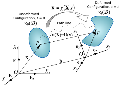
Figure 1. Motion of a continuum body.
A change in the configuration of a continuum body results in a displacement. The displacement of a body has two components: a rigid-body displacement and a deformation. A rigid-body displacement consists of a simultaneous translation and rotation of the body without changing its shape or size. Deformation implies the change in shape and/or size of the body from an initial or undeformed configuration κ0(B) to a current or deformed configuration κt(B) (Figure 1).
If after a displacement of the continuum there is a relative displacement between particles, a deformation has occurred. On the other hand, if after displacement of the continuum the relative displacement between particles in the current configuration is zero, then there is no deformation and a rigid-body displacement is said to have occurred.
The vector joining the positions of a particle P in the undeformed configuration and deformed configuration is called the displacement vector u(X,t) = uiei in the Lagrangian description, or U(x,t) = UJEJ in the Eulerian description.
A displacement field is a vector field of all displacement vectors for all particles in the body, which relates the deformed configuration with the undeformed configuration. It is convenient to do the analysis of deformation or motion of a continuum body in terms of the displacement field. In general, the displacement field is expressed in terms of the material coordinates as
- u(X,t)=b(X,t)+x(X,t)−Xorui=αiJbJ+xi−αiJXJdisplaystyle mathbf u (mathbf X ,t)=mathbf b (mathbf X ,t)+mathbf x (mathbf X ,t)-mathbf X qquad textorqquad u_i=alpha _iJb_J+x_i-alpha _iJX_J

or in terms of the spatial coordinates as
- U(x,t)=b(x,t)+x−X(x,t)orUJ=bJ+αJixi−XJdisplaystyle mathbf U (mathbf x ,t)=mathbf b (mathbf x ,t)+mathbf x -mathbf X (mathbf x ,t)qquad textorqquad U_J=b_J+alpha _Jix_i-X_J,

where αJi are the direction cosines between the material and spatial coordinate systems with unit vectors EJ and ei, respectively. Thus
- EJ⋅ei=αJi=αiJdisplaystyle mathbf E _Jcdot mathbf e _i=alpha _Ji=alpha _iJ

and the relationship between ui and UJ is then given by
- ui=αiJUJorUJ=αJiuidisplaystyle u_i=alpha _iJU_Jqquad textorqquad U_J=alpha _Jiu_i

Knowing that
- ei=αiJEJdisplaystyle mathbf e _i=alpha _iJmathbf E _J

then
- u(X,t)=uiei=ui(αiJEJ)=UJEJ=U(x,t)displaystyle mathbf u (mathbf X ,t)=u_imathbf e _i=u_i(alpha _iJmathbf E _J)=U_Jmathbf E _J=mathbf U (mathbf x ,t)

It is common to superimpose the coordinate systems for the undeformed and deformed configurations, which results in b = 0, and the direction cosines become Kronecker deltas:
- EJ⋅ei=δJi=δiJdisplaystyle mathbf E _Jcdot mathbf e _i=delta _Ji=delta _iJ

Thus, we have
- u(X,t)=x(X,t)−Xorui=xi−δiJXJ=xi−Xidisplaystyle mathbf u (mathbf X ,t)=mathbf x (mathbf X ,t)-mathbf X qquad textorqquad u_i=x_i-delta _iJX_J=x_i-X_i

or in terms of the spatial coordinates as
- U(x,t)=x−X(x,t)orUJ=δJixi−XJ=xJ−XJdisplaystyle mathbf U (mathbf x ,t)=mathbf x -mathbf X (mathbf x ,t)qquad textorqquad U_J=delta _Jix_i-X_J=x_J-X_J

Displacement gradient tensor
The partial differentiation of the displacement vector with respect to the material coordinates yields the material displacement gradient tensor ∇XU. Thus we have:
u(X,t)=x(X,t)−X∇Xu=∇Xx−I∇Xu=F−Idisplaystyle beginalignedmathbf u (mathbf X ,t)&=mathbf x (mathbf X ,t)-mathbf X \nabla _mathbf X mathbf u &=nabla _mathbf X mathbf x -mathbf I \nabla _mathbf X mathbf u &=mathbf F -mathbf I \endalignedor
ui=xi−δiJXJ=xi−Xi∂ui∂XK=∂xi∂XK−δiKdisplaystyle beginalignedu_i&=x_i-delta _iJX_J=x_i-X_i\frac partial u_ipartial X_K&=frac partial x_ipartial X_K-delta _iK\endaligned


where F is the deformation gradient tensor.
Similarly, the partial differentiation of the displacement vector with respect to the spatial coordinates yields the spatial displacement gradient tensor ∇xU. Thus we have,
U(x,t)=x−X(x,t)∇xU=I−∇xX∇xU=I−F−1displaystyle beginalignedmathbf U (mathbf x ,t)&=mathbf x -mathbf X (mathbf x ,t)\nabla _mathbf x mathbf U &=mathbf I -nabla _mathbf x mathbf X \nabla _mathbf x mathbf U &=mathbf I -mathbf F ^-1\endalignedor
UJ=δJixi−XJ=xJ−XJ∂UJ∂xk=δJk−∂XJ∂xkdisplaystyle beginalignedU_J&=delta _Jix_i-X_J=x_J-X_J\frac partial U_Jpartial x_k&=delta _Jk-frac partial X_Jpartial x_k\endaligned


Examples of deformations
Homogeneous (or affine) deformations are useful in elucidating the behavior of materials. Some homogeneous deformations of interest are
- uniform extension
- pure dilation
- equibiaxial tension
- simple shear
- pure shear
Plane deformations are also of interest, particularly in the experimental context.
Plane deformation
A plane deformation, also called plane strain, is one where the deformation is restricted to one of the planes in the reference configuration. If the deformation is restricted to the plane described by the basis vectors e1, e2, the deformation gradient has the form
- F=F11e1⊗e1+F12e1⊗e2+F21e2⊗e1+F22e2⊗e2+e3⊗e3displaystyle boldsymbol F=F_11mathbf e _1otimes mathbf e _1+F_12mathbf e _1otimes mathbf e _2+F_21mathbf e _2otimes mathbf e _1+F_22mathbf e _2otimes mathbf e _2+mathbf e _3otimes mathbf e _3

In matrix form,
- F=[F11F120F21F220001]displaystyle boldsymbol F=beginbmatrixF_11&F_12&0\F_21&F_22&0\0&0&1endbmatrix

From the polar decomposition theorem, the deformation gradient, up to a change of coordinates, can be decomposed into a stretch and a rotation. Since all the deformation is in a plane, we can write[8]
- F=R⋅U=[cosθsinθ0−sinθcosθ0001][λ1000λ20001]displaystyle boldsymbol F=boldsymbol Rcdot boldsymbol U=beginbmatrixcos theta &sin theta &0\-sin theta &cos theta &0\0&0&1endbmatrixbeginbmatrixlambda _1&0&0\0&lambda _2&0\0&0&1endbmatrix

where θ is the angle of rotation and λ1, λ2 are the principal stretches.
Isochoric plane deformation
If the deformation is isochoric (volume preserving) then det(F) = 1 and we have
- F11F22−F12F21=1displaystyle F_11F_22-F_12F_21=1

Alternatively,
- λ1λ2=1displaystyle lambda _1lambda _2=1

Simple shear
A simple shear deformation is defined as an isochoric plane deformation in which there is a set of line elements with a given reference orientation that do not change length and orientation during the deformation.[8]
If e1 is the fixed reference orientation in which line elements do not deform during the deformation then λ1 = 1 and F·e1 = e1.
Therefore,
- F11e1+F21e2=e1⟹F11=1 ; F21=0displaystyle F_11mathbf e _1+F_21mathbf e _2=mathbf e _1quad implies quad F_11=1~;~~F_21=0

Since the deformation is isochoric,
- F11F22−F12F21=1⟹F22=1displaystyle F_11F_22-F_12F_21=1quad implies quad F_22=1

Define
- γ:=F12displaystyle gamma :=F_12,

Then, the deformation gradient in simple shear can be expressed as
- F=[1γ0010001]displaystyle boldsymbol F=beginbmatrix1&gamma &0\0&1&0\0&0&1endbmatrix

Now,
- F⋅e2=F12e1+F22e2=γe1+e2⟹F⋅(e2⊗e2)=γe1⊗e2+e2⊗e2displaystyle boldsymbol Fcdot mathbf e _2=F_12mathbf e _1+F_22mathbf e _2=gamma mathbf e _1+mathbf e _2quad implies quad boldsymbol Fcdot (mathbf e _2otimes mathbf e _2)=gamma mathbf e _1otimes mathbf e _2+mathbf e _2otimes mathbf e _2

Since
- ei⊗ei=1displaystyle mathbf e _iotimes mathbf e _i=boldsymbol mathit 1

we can also write the deformation gradient as
- F=1+γe1⊗e2displaystyle boldsymbol F=boldsymbol mathit 1+gamma mathbf e _1otimes mathbf e _2

See also
- Euler–Bernoulli beam theory
- Deformation (engineering)
- Finite strain theory
- Infinitesimal strain theory
- Moiré pattern
- Shear modulus
- Shear stress
- Shear strength
- Stress (mechanics)
- Stress measures
References
^ Truesdell, C.; Noll, W. (2004). The non-linear field theories of mechanics (3rd ed.). Springer. p. 48..mw-parser-output cite.citationfont-style:inherit.mw-parser-output qquotes:"""""""'""'".mw-parser-output code.cs1-codecolor:inherit;background:inherit;border:inherit;padding:inherit.mw-parser-output .cs1-lock-free abackground:url("//upload.wikimedia.org/wikipedia/commons/thumb/6/65/Lock-green.svg/9px-Lock-green.svg.png")no-repeat;background-position:right .1em center.mw-parser-output .cs1-lock-limited a,.mw-parser-output .cs1-lock-registration abackground:url("//upload.wikimedia.org/wikipedia/commons/thumb/d/d6/Lock-gray-alt-2.svg/9px-Lock-gray-alt-2.svg.png")no-repeat;background-position:right .1em center.mw-parser-output .cs1-lock-subscription abackground:url("//upload.wikimedia.org/wikipedia/commons/thumb/a/aa/Lock-red-alt-2.svg/9px-Lock-red-alt-2.svg.png")no-repeat;background-position:right .1em center.mw-parser-output .cs1-subscription,.mw-parser-output .cs1-registrationcolor:#555.mw-parser-output .cs1-subscription span,.mw-parser-output .cs1-registration spanborder-bottom:1px dotted;cursor:help.mw-parser-output .cs1-hidden-errordisplay:none;font-size:100%.mw-parser-output .cs1-visible-errorfont-size:100%.mw-parser-output .cs1-subscription,.mw-parser-output .cs1-registration,.mw-parser-output .cs1-formatfont-size:95%.mw-parser-output .cs1-kern-left,.mw-parser-output .cs1-kern-wl-leftpadding-left:0.2em.mw-parser-output .cs1-kern-right,.mw-parser-output .cs1-kern-wl-rightpadding-right:0.2em
^ Wu, H.-C. (2005). Continuum Mechanics and Plasticity. CRC Press. ISBN 1-58488-363-4.
^ Lubliner, Jacob (2008). Plasticity Theory (PDF) (Revised ed.). Dover Publications. ISBN 0-486-46290-0. Archived from the original (PDF) on 2010-03-31.
^ ab Rees, David (2006). Basic Engineering Plasticity: An Introduction with Engineering and Manufacturing Applications. Butterworth-Heinemann. ISBN 0-7506-8025-3. Archived from the original on 2017-12-22.
^ "Earth."Encyclopædia Britannica from Encyclopædia Britannica 2006 Ultimate Reference Suite DVD .[2009].
^ Rees, David (2006). Basic Engineering Plasticity: An Introduction with Engineering and Manufacturing Applications. Butterworth-Heinemann. p. 41. ISBN 0-7506-8025-3. Archived from the original on 2017-12-22.
^ Hencky, H. (1928). "Über die Form des Elastizitätsgesetzes bei ideal elastischen Stoffen". Zeitschrift für technische Physik. 9: 215–220.
^ abc Ogden, R. W. (1984). Non-linear Elastic Deformations. Dover.
Further reading
Bazant, Zdenek P.; Cedolin, Luigi (2010). Three-Dimensional Continuum Instabilities and Effects of Finite Strain Tensor, chapter 11 in "Stability of Structures", 3rd ed. Singapore, New Jersey, London: World Scientific Publishing. ISBN 9814317039.
Dill, Ellis Harold (2006). Continuum Mechanics: Elasticity, Plasticity, Viscoelasticity. Germany: CRC Press. ISBN 0-8493-9779-0.
Hutter, Kolumban; Jöhnk, Klaus (2004). Continuum Methods of Physical Modeling. Germany: Springer. ISBN 3-540-20619-1.
Jirasek, M; Bazant, Z.P. (2002). Inelastic Analysis of Structures. London and New York: J. Wiley & Sons. ISBN 0471987166.
Lubarda, Vlado A. (2001). Elastoplasticity Theory. CRC Press. ISBN 0-8493-1138-1.
Macosko, C. W. (1994). Rheology: principles, measurement and applications. VCH Publishers. ISBN 1-56081-579-5.
Mase, George E. (1970). Continuum Mechanics. McGraw-Hill Professional. ISBN 0-07-040663-4.
Mase, G. Thomas; Mase, George E. (1999). Continuum Mechanics for Engineers (2nd ed.). CRC Press. ISBN 0-8493-1855-6.
Nemat-Nasser, Sia (2006). Plasticity: A Treatise on Finite Deformation of Heterogeneous Inelastic Materials. Cambridge: Cambridge University Press. ISBN 0-521-83979-3.
Prager, William (1961). Introduction to Mechanics of Continua. Boston: Ginn and Co. ISBN 0486438090.


