Odtnhj

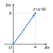
A complex number can be visually represented as a pair of numbers (a, b) forming a vector on a diagram called an Argand diagram, representing the complex plane. "Re" is the real axis, "Im" is the imaginary axis, and i satisfies i² = −1.

A complex number is a number that can be expressed in the form a + bi, where a and b are real numbers, and i is a solution of the equation x² = −1. Because no real number satisfies this equation, i is called an imaginary number. For the complex number a + bi, a is called the real part, and b is called the imaginary part. Despite the historical nomenclature "imaginary", complex numbers are regarded in the mathematical sciences as just as "real" as the real numbers, and are fundamental in many aspects of the scientific description of the natural world.^[1][2]

The complex number system can be defined as the algebraic extension of the ordinary real numbers by an imaginary number i.^[3] This means that complex numbers can be added, subtracted, and multiplied, as polynomials in the variable i, with the rule i² = −1 imposed. Furthermore, complex numbers can also be divided by nonzero complex numbers. Overall, the complex number system is a field.

The complex numbers give rise to the fundamental theorem of algebra: every non-constant polynomial equation with complex coefficients has a complex solution. This property is true of the complex numbers, but not the reals. The 16th century Italian mathematician Gerolamo Cardano is credited with introducing complex numbers in his attempts to find solutions to cubic equations.^[4]

Geometrically, complex numbers extend the concept of the one-dimensional number line to the two-dimensional complex plane by using the horizontal axis for the real part and the vertical axis for the imaginary part. The complex number a + bi can be identified with the point (a, b) in the complex plane. A complex number whose real part is zero is said to be purely imaginary; the points for these numbers lie on the vertical axis of the complex plane. A complex number whose imaginary part is zero can be viewed as a real number; its point lies on the horizontal axis of the complex plane. Complex numbers can also be represented in polar form, which associates each complex number with its distance from the origin (its magnitude) and with a particular angle known as the argument of this complex number.

Overview

Complex numbers allow solutions to certain equations that have no solutions in real numbers. For example, the equation

(x+1)2=−9displaystyle (x+1)^2=-9

has no real solution, since the square of a real number cannot be negative. Complex numbers provide a solution to this problem. The idea is to extend the real numbers with an indeterminate i (sometimes called the imaginary unit) that is taken to satisfy the relation i² = −1, so that solutions to equations like the preceding one can be found. In this case the solutions are −1 + 3i and −1 − 3i, as can be verified using the fact that i² = −1:

((−1+3i)+1)2=(3i)2=(32)(i2)=9(−1)=−9,displaystyle ((-1+3i)+1)^2=(3i)^2=left(3^2right)left(i^2right)=9(-1)=-9,

((−1−3i)+1)2=(−3i)2=(−3)2(i2)=9(−1)=−9.displaystyle ((-1-3i)+1)^2=(-3i)^2=(-3)^2left(i^2right)=9(-1)=-9.

According to the fundamental theorem of algebra, all polynomial equations with real or complex coefficients in a single variable have a solution in complex numbers.

Definition

An illustration of the complex plane. The real part of a complex number z = x + iy is x, and its imaginary part is y.

A complex number is a number of the form a + bi, where a and b are real numbers and i is an indeterminate satisfying i² = −1. For example, 2 + 3i is a complex number.^[5]

A complex number may therefore be defined as a polynomial in the single indeterminate i, with the relation i² + 1 = 0 imposed. From this definition, complex numbers can be added or multiplied, using the addition and multiplication for polynomials. Formally, the set of complex numbers is the quotient ring of the polynomial ring in the indeterminate i, by the ideal generated by the polynomial i² + 1 (see below).^[6] The set of all complex numbers is denoted by Cdisplaystyle mathbf C (upright bold) or Cdisplaystyle mathbb C (blackboard bold).

The real number a is called the real part of the complex number a + bi; the real number b is called the imaginary part of a + bi. By this convention, the imaginary part does not include a factor of i: hence b, not bi, is the imaginary part.^[7][8] The real part of a complex number z is denoted by Re(z) or ℜ(z); the imaginary part of a complex number z is denoted by Im(z) or ℑ(z). For example,

Re⁡(2+3i)=2Im⁡(2+3i)=3.displaystyle beginalignedoperatorname Re (2+3i)&=2\operatorname Im (2+3i)&=3.endaligned

A real number a can be regarded as a complex number a + 0i whose imaginary part is 0. A purely imaginary number bi is a complex number 0 + bi whose real part is zero. It is common to write a for a + 0i and bi for 0 + bi. Moreover, when the imaginary part is negative, it is common to write a − bi with b > 0 instead of a + (−b)i, for example 3 − 4i instead of 3 + (−4)i.

Cartesian form and definition via ordered pairs

A complex number can thus be identified with an ordered pair (Re(z), Im(z)) in the Cartesian plane, an identification sometimes known as the Cartesian form of z. In fact, a complex number can be defined as an ordered pair (a, b), but then rules for addition and multiplication must also be included as part of the definition (see below).^[9]William Rowan Hamilton introduced this approach to define the complex number system.^[10]

Complex plane

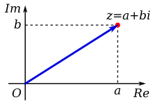
Figure 1: A complex number z, plotted as a point (red) and position vector (blue) on an Argand diagram; a + bi is its rectangular expression.

A complex number can be viewed as a point or position vector in a two-dimensional Cartesian coordinate system called the complex plane or Argand diagram (see Pedoe 1988 and Solomentsev 2001), named after Jean-Robert Argand. The numbers are conventionally plotted using the real part as the horizontal component, and imaginary part as vertical (see Figure 1). These two values used to identify a given complex number are therefore called its Cartesian, rectangular, or algebraic form.

A position vector may also be defined in terms of its magnitude and direction relative to the origin. These are emphasized in a complex number's polar form. Using the polar form of the complex number in calculations may lead to a more intuitive interpretation of mathematical results. Notably, the operations of addition and multiplication take on a very natural geometric character when complex numbers are viewed as position vectors: addition corresponds to vector addition while multiplication corresponds to multiplying their magnitudes and adding their arguments (i.e. the angles they make with the x axis). Viewed in this way the multiplication of a complex number by i corresponds to rotating the position vector counterclockwise by a quarter turn (90°) about the origin: (a + bi)i = ai + bi² = −b + ai.

History in brief

Main section: History

The solution in radicals (without trigonometric functions) of a general cubic equation contains the square roots of negative numbers when all three roots are real numbers, a situation that cannot be rectified by factoring aided by the rational root test if the cubic is irreducible (the so-called casus irreducibilis). This conundrum led Italian mathematician Gerolamo Cardano to conceive of complex numbers in around 1545,^[11] though his understanding was rudimentary.

Work on the problem of general polynomials ultimately led to the fundamental theorem of algebra, which shows that with complex numbers, a solution exists to every polynomial equation of degree one or higher. Complex numbers thus form an algebraically closed field, where any polynomial equation has a root.

Many mathematicians contributed to the full development of complex numbers. The rules for addition, subtraction, multiplication, and division of complex numbers were developed by the Italian mathematician Rafael Bombelli.^[12] A more abstract formalism for the complex numbers was further developed by the Irish mathematician William Rowan Hamilton, who extended this abstraction to the theory of quaternions.

Notation

Because it is a polynomial in the indeterminate i, a + ib may be written instead of a + bi, which is often expedient when b is a radical.^[13] In some disciplines, in particular electromagnetism and electrical engineering, j is used instead of i,^[14] since i is frequently used for electric current. In these cases complex numbers are written as a + bj or a + jb.

Equality and order relations

Two complex numbers are equal if and only if both their real and imaginary parts are equal. That is, complex numbers z1displaystyle z_1 and z2displaystyle z_2 are equal if and only if
Re⁡(z1)=Re⁡(z2)displaystyle operatorname Re (z_1)=operatorname Re (z_2) and Im⁡(z1)=Im⁡(z2)displaystyle operatorname Im (z_1)=operatorname Im (z_2). If the complex numbers are written in polar form, they are equal if and only if they have the same argument and the same magnitude.

Because complex numbers are naturally thought of as existing on a two-dimensional plane, there is no natural linear ordering on the set of complex numbers. Furthermore, there is no linear ordering on the complex numbers that is compatible with addition and multiplication – the complex numbers cannot have the structure of an ordered field. This is because any square in an ordered field is at least 0, but i² = −1.

Elementary operations

Conjugate

Geometric representation of z and its conjugate z¯displaystyle overline z in the complex plane

The complex conjugate of the complex number z = x + yi is given by x − yi. It is denoted by either z¯displaystyle overline z or z*.^[15] This unary operation on complex numbers cannot be expressed by applying only their basic operations addition, subtraction, multiplication and division.

Geometrically, z¯displaystyle overline z is the "reflection" of z about the real axis. Conjugating twice gives the original complex number

z¯¯=z,displaystyle overline overline z=z,

which makes this operation an involution. The reflection leaves both the real part and the magnitude of zdisplaystyle z unchanged, that is

Re⁡(z¯)=Re⁡(z)displaystyle operatorname Re (overline z)=operatorname Re (z)quad and |z¯|=|z|..

The imaginary part and the argument of a complex number zdisplaystyle z change their sign under conjugation

Im⁡(z¯)=−Im⁡(z)displaystyle operatorname Im (overline z)=-operatorname Im (z)quad and arg⁡(z¯)≡−arg⁡(z)(mod2π).displaystyle quad operatorname arg (overline z)equiv -operatorname arg (z)pmod 2pi .

For details on argument and magnitude see #Polar form.

The product of a complex number z=x+yidisplaystyle z=x+yi and its conjugate is always a positive real number and equals the square of the magnitude of each:

z⋅z¯=x2+y2.displaystyle zcdot overline z=x^2+y^2.

This property can be used used to convert a fraction with a complex denominator to an equivalent fraction with a real denominator by expanding both numerator and denominator of the fraction by the conjugate of the given denominator. This process is sometimes called "rationalization" of the denominator (although the denominator in the final expression might be an irrational real number), because it resembles the method to remove roots from simple expressions in a denominator.

The real and imaginary parts of a complex number z can be extracted using the conjugation:

Re⁡(z)=z+z¯2,displaystyle operatorname Re (z)=dfrac z+overline z2,quad and Im⁡(z)=z−z¯2i.displaystyle quad operatorname Im (z)=dfrac z-overline z2i.

Moreover, a complex number is real if and only if it equals its own conjugate.

Conjugation distributes over the basic complex arithmetic operations:

z±w¯=z¯±w¯,displaystyle overline zpm w=overline zpm overline w,

z⋅w¯=z¯⋅w¯,z/w¯=z¯/w¯.displaystyle overline zcdot w=overline zcdot overline w,quad overline z/w=overline z/overline w.

Conjugation is also employed in Inversive geometry, a branch of geometry studying reflections more general than ones about a line. In the network analysis of electrical circuits, the complex conjugate is used in finding the equivalent impedance when the maximum power transfer theorem is looked for.

Addition and subtraction

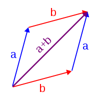
Addition of two complex numbers can be done geometrically by constructing a parallelogram.

Two complex numbers adisplaystyle a and bdisplaystyle b are most easily added by separately adding their real and imaginary parts of the summands. That is to say:

a+b=(x+yi)+(u+vi)=(x+u)+(y+v)i.displaystyle a+b=(x+yi)+(u+vi)=(x+u)+(y+v)i.

Similarly, subtraction can be performed as

a−b=(x+yi)−(u+vi)=(x−u)+(y−v)i.displaystyle a-b=(x+yi)-(u+vi)=(x-u)+(y-v)i.

Using the visualization of complex numbers in the complex plane, the addition has the following geometric interpretation: the sum of two complex numbers adisplaystyle a and bdisplaystyle b, interpreted as points in the complex plane, is the point obtained by building a parallelogram from the three vertices Odisplaystyle O, and the points of the arrows labeled adisplaystyle a and bdisplaystyle b (provided that they are not on a line). Equivalently, calling these points A,B,displaystyle A,;B, respectively and the fourth point of the parallelogram X,displaystyle X, the triangles OABdisplaystyle OAB and XBAdisplaystyle XBA are congruent. A visualization of the subtraction can be achieved by considering addition of the negative subtrahend.

Multiplication

Since the real part, the imaginary part, and the indeterminate idisplaystyle i in a complex number are all considered as numbers in themselves, two complex numbers, given as z=x+yidisplaystyle z=x+yi and w=u+vidisplaystyle w=u+vi are multiplied under the rules of the distributive property, the commutative properties and the defining property i2=−1displaystyle i^2=-1 in the following way

z⋅w=(x+yi)⋅(u+vi)=x(u+vi)+yi(u+vi)by the (right) distributive law=xu+xvi+yiu+yiviby the (left) distributive law=xu+yivi+xvi+yiuby the commutativity of addition=xu+yvi2+xvi+yuiby the commutativity of multiplication=(xu+yvi2)+(xvi+yui)by the associativity of addition=(xu−yv)+(xvi+yui)by the defining property of i=(xu−yv)+(xv+yu)iby the distributive law.displaystyle beginalignedzcdot w&=(x+yi)cdot (u+vi)&\&=x(u+vi)+yi(u+vi)&&textby the (right) distributive law\&=xu+xvi+yiu+yivi&&textby the (left) distributive law\&=xu+yivi+xvi+yiu&&textby the commutativity of addition\&=xu+yvi^2+xvi+yui&&textby the commutativity of multiplication\&=(xu+yvi^2)+(xvi+yui)&&textby the associativity of addition\&=(xu-yv)+(xvi+yui)&&textby the defining property of i\&=(xu-yv)+(xv+yu)i&&textby the distributive law.endaligned

Reciprocal and division

Using the conjugation, the reciprocal of a nonzero complex number z = x + yi can always be broken down to

1z=z¯zz¯=z¯|z|2=z¯x2+y2=xx2+y2−yx2+y2i,displaystyle frac 1z=frac overline zzoverline z=frac overline z=frac overline zx^2+y^2=frac xx^2+y^2-frac yx^2+y^2i,

since non-zero implies that x2+y2displaystyle x^2+y^2 is greater than zero.

This can be used to express a division of an arbitrary complex number w=u+vidisplaystyle w=u+vi by a non-zero complex number zdisplaystyle z as

wz=w⋅1z=(u+vi)⋅(xx2+y2−yx2+y2i)=1x2+y2((ux+vy)+(vx−uy)i).displaystyle frac wz=wcdot frac 1z=(u+vi)cdot left(frac xx^2+y^2-frac yx^2+y^2iright)=frac 1x^2+y^2left((ux+vy)+(vx-uy)iright).

Square root

The square roots of a + bi (with b ≠ 0) are ±(γ+δi)displaystyle pm (gamma +delta i), where

γ=a+a2+b22displaystyle gamma =sqrt frac a+sqrt a^2+b^22

and

δ=sgn⁡(b)−a+a2+b22,displaystyle delta =operatorname sgn (b)sqrt frac -a+sqrt a^2+b^22,

where sgn is the signum function. This can be seen by squaring ±(γ+δi)displaystyle pm (gamma +delta i) to obtain a + bi.^[16][17] Here a2+b2displaystyle sqrt a^2+b^2 is called the modulus of a + bi, and the square root sign indicates the square root with non-negative real part, called the principal square root; also a2+b2=zz¯,displaystyle sqrt a^2+b^2=sqrt zoverline z, where z=a+bi.displaystyle z=a+bi.^[18]

Polar form

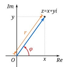
Figure 2: The argument φ and modulus r locate a point on an Argand diagram; r(cos⁡φ+isin⁡φ)displaystyle r(cos varphi +isin varphi ) or reiφdisplaystyle re^ivarphi are polar expressions of the point.

Absolute value and argument

An alternative way of defining a point P in the complex plane, other than using the x- and y-coordinates, is to use the distance of the point from O, the point whose coordinates are (0, 0) (the origin), together with the angle subtended between the positive real axis and the line segment OP in a counterclockwise direction. This idea leads to the polar form of complex numbers.

The absolute value (or modulus or magnitude) of a complex number z = x + yi is^[19]

r=|z|=x2+y2.displaystyle r=

If z is a real number (that is, if y = 0), then r = |x|. That is, the absolute value of a real number equals its absolute value as a complex number.

By Pythagoras' theorem, the absolute value of complex number is the distance to the origin of the point representing the complex number in the complex plane.

The square of the absolute value is

|z|2=zz¯=x2+y2.z

where z¯displaystyle overline z is the complex conjugate of z.displaystyle z.

The argument of z (in many applications referred to as the "phase") is the angle of the radius OP with the positive real axis, and is written as arg⁡(z)displaystyle arg(z). As with the modulus, the argument can be found from the rectangular form x+yidisplaystyle x+yi:^[20]

φ=arg⁡(z)={arctan⁡(yx)if x>0arctan⁡(yx)+πif x<0 and y≥0arctan⁡(yx)−πif x<0 and y<0π2if x=0 and y>0−π2if x=0 and y<0indeterminate if x=0 and y=0.displaystyle varphi =arg(z)=begincasesarctan left(dfrac yxright)&textif x>0\arctan left(dfrac yxright)+pi &textif x<0text and ygeq 0\arctan left(dfrac yxright)-pi &textif x<0text and y<0\dfrac pi 2&textif x=0text and y>0\-dfrac pi 2&textif x=0text and y<0\textindeterminate &textif x=0text and y=0.endcases

Visualisation of the square to sixth roots of a complex number z, in polar form re^iφ where φ = arg z and r = |z | – if z is real, φ = 0 or π. Principal roots are in black.

Normally, as given above, the principal value in the interval (−π, π] is chosen. Values in the range [0, 2π) are obtained by adding 2π if the value is negative. The value of φ is expressed in radians in this article. It can increase by any integer multiple of 2π and still give the same angle. Hence, the arg function is sometimes considered as multivalued. The polar angle for the complex number 0 is indeterminate, but arbitrary choice of the angle 0 is common.

The value of φ equals the result of atan2:

φ=atan2⁡(Im⁡(z),Re⁡(z)).displaystyle varphi =operatorname atan2 left(operatorname Im (z),operatorname Re (z)right).

Together, r and φ give another way of representing complex numbers, the polar form, as the combination of modulus and argument fully specify the position of a point on the plane. Recovering the original rectangular co-ordinates from the polar form is done by the formula called trigonometric form

z=r(cos⁡φ+isin⁡φ).displaystyle z=r(cos varphi +isin varphi ).

Using Euler's formula this can be written as

z=reiφ.displaystyle z=re^ivarphi .

Using the cis function, this is sometimes abbreviated to

z=rcis⁡φ.displaystyle z=roperatorname cis varphi .

In angle notation, often used in electronics to represent a phasor with amplitude r and phase φ, it is written as^[21]

z=r∠φ.displaystyle z=rangle varphi .

Multiplication and division in polar form

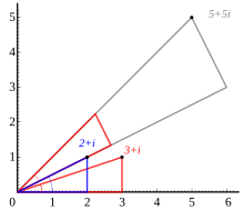
Multiplication of 2 + i (blue triangle) and 3 + i (red triangle). The red triangle is rotated to match the vertex of the blue one and stretched by √5, the length of the hypotenuse of the blue triangle.

Formulas for multiplication, division and exponentiation are simpler in polar form than the corresponding formulas in Cartesian coordinates. Given two complex numbers z₁ = r₁(cos φ₁ + i sin φ₁) and z₂ = r₂(cos φ₂ + i sin φ₂), because of the trigonometric identities

cos⁡(a)cos⁡(b)−sin⁡(a)sin⁡(b)=cos⁡(a+b)displaystyle cos(a)cos(b)-sin(a)sin(b)=cos(a+b)

cos⁡(a)sin⁡(b)+sin⁡(a)cos⁡(b)=sin⁡(a+b)displaystyle cos(a)sin(b)+sin(a)cos(b)=sin(a+b)

we may derive

z1z2=r1r2(cos⁡(φ1+φ2)+isin⁡(φ1+φ2)).displaystyle z_1z_2=r_1r_2(cos(varphi _1+varphi _2)+isin(varphi _1+varphi _2)).

In other words, the absolute values are multiplied and the arguments are added to yield the polar form of the product. For example, multiplying by i corresponds to a quarter-turn counter-clockwise, which gives back i² = −1. The picture at the right illustrates the multiplication of

(2+i)(3+i)=5+5i.displaystyle (2+i)(3+i)=5+5i.

Since the real and imaginary part of 5 + 5i are equal, the argument of that number is 45 degrees, or π/4 (in radian). On the other hand, it is also the sum of the angles at the origin of the red and blue triangles are arctan(1/3) and arctan(1/2), respectively. Thus, the formula

π4=arctan⁡(12)+arctan⁡(13)displaystyle frac pi 4=arctan left(frac 12right)+arctan left(frac 13right)

holds. As the arctan function can be approximated highly efficiently, formulas like this—known as Machin-like formulas—are used for high-precision approximations of π.

Similarly, division is given by

z1z2=r1r2(cos⁡(φ1−φ2)+isin⁡(φ1−φ2)).displaystyle frac z_1z_2=frac r_1r_2left(cos(varphi _1-varphi _2)+isin(varphi _1-varphi _2)right).

Exponentiation

Euler's formula

Euler's formula states that, for any real number x,

eix=cos⁡x+isin⁡x displaystyle e^ix=cos x+isin x ,

where e is the base of the natural logarithm. This can be proved through induction by observing that

i0=1,i1=i,i2=−1,i3=−i,i4=1,i5=i,i6=−1,i7=−i,displaystyle beginalignedi^0&=1,quad &i^1&=i,quad &i^2&=-1,quad &i^3&=-i,\i^4&=1,quad &i^5&=i,quad &i^6&=-1,quad &i^7&=-i,endaligned

and so on, and by considering the Taylor series expansions of e^ix, cos x and sin x:

eix=1+ix+(ix)22!+(ix)33!+(ix)44!+(ix)55!+(ix)66!+(ix)77!+(ix)88!+⋯=1+ix−x22!−ix33!+x44!+ix55!−x66!−ix77!+x88!+⋯=(1−x22!+x44!−x66!+x88!−⋯)+i(x−x33!+x55!−x77!+⋯)=cos⁡x+isin⁡x .displaystyle beginalignede^ix&=1+ix+frac (ix)^22!+frac (ix)^33!+frac (ix)^44!+frac (ix)^55!+frac (ix)^66!+frac (ix)^77!+frac (ix)^88!+cdots \[8pt]&=1+ix-frac x^22!-frac ix^33!+frac x^44!+frac ix^55!-frac x^66!-frac ix^77!+frac x^88!+cdots \[8pt]&=left(1-frac x^22!+frac x^44!-frac x^66!+frac x^88!-cdots right)+ileft(x-frac x^33!+frac x^55!-frac x^77!+cdots right)\[8pt]&=cos x+isin x .endaligned

The rearrangement of terms is justified because each series is absolutely convergent.

Natural logarithm

It follows from Euler's formula that, for any complex number z written in polar form,

z=r(cos⁡φ+isin⁡φ)displaystyle z=r(cos varphi +isin varphi )

where r is a non-negative real number, one possible value for the complex logarithm of z is

ln⁡(z)=ln⁡(r)+φi.displaystyle ln(z)=ln(r)+varphi i.

Because cosine and sine are periodic functions, other possible values may be obtained. For example, eiπ=e3iπ=−1displaystyle e^ipi =e^3ipi =-1, so both iπdisplaystyle ipi and 3iπdisplaystyle 3ipi are two possible values for the natural logarithm of −1displaystyle -1.

To deal with the existence of more than one possible value for a given input, the complex logarithm may be considered a multi-valued function, with

ln⁡(z)=ln⁡(r)+(φ+2πk)i∣k∈Z.displaystyle ln(z)=leftln(r)+(varphi +2pi k)imid kin mathbb Z right.

Alternatively, a branch cut can be used to define a single-valued "branch" of the complex logarithm.

Integer and fractional exponents

We may use the identity

ln⁡(ab)=bln⁡(a)displaystyle ln left(a^bright)=bln(a)

to define complex exponentiation, which is likewise multi-valued:

ln⁡(zn)=ln⁡((r(cos⁡φ+isin⁡φ))n)=nln⁡(r(cos⁡φ+isin⁡φ))= k∈Z= k∈Z.displaystyle beginalignedln(z^n)&=ln((r(cos varphi +isin varphi ))^n)\&=nln(r(cos varphi +isin varphi ))\&=n(ln(r)+(varphi +k2pi )i) \&= kin mathbb Z .endaligned

When n is an integer, this simplifies to de Moivre's formula:

zn=(r(cos⁡φ+isin⁡φ))n=rn⋅(cos⁡nφ+isin⁡nφ).displaystyle z^n=(r(cos varphi +isin varphi ))^n=r^ncdot (cos nvarphi +isin nvarphi ).

The nth roots of z are given by

zn=rn(cos⁡(φ+2kπn)+isin⁡(φ+2kπn))displaystyle sqrt[n]z=sqrt[n]rleft(cos left(frac varphi +2kpi nright)+isin left(frac varphi +2kpi nright)right)

for any integer k satisfying 0 ≤ k ≤ n − 1. Here ⁿ√r is the usual (positive) nth root of the positive real number r. While the nth root of a positive real number r is chosen to be the positive real number c satisfying cⁿ = r there is no natural way of distinguishing one particular complex nth root of a complex number. Therefore, the nth root of z is considered as a multivalued function (in z), as opposed to a usual function f, for which f(z) is a uniquely defined number. Formulas such as

znn=zdisplaystyle sqrt[n]z^n=z

(which holds for positive real numbers), do in general not hold for complex numbers.

Properties

Field structure

The set C of complex numbers is a field.^[22] Briefly, this means that the following facts hold: first, any two complex numbers can be added and multiplied to yield another complex number. Second, for any complex number z, its additive inverse −z is also a complex number; and third, every nonzero complex number has a reciprocal complex number. Moreover, these operations satisfy a number of laws, for example the law of commutativity of addition and multiplication for any two complex numbers z₁ and z₂:

z1+z2=z2+z1,displaystyle z_1+z_2=z_2+z_1,

z1z2=z2z1.displaystyle z_1z_2=z_2z_1.

These two laws and the other requirements on a field can be proven by the formulas given above, using the fact that the real numbers themselves form a field.

Unlike the reals, C is not an ordered field, that is to say, it is not possible to define a relation z₁ < z₂ that is compatible with the addition and multiplication. In fact, in any ordered field, the square of any element is necessarily positive, so i² = −1 precludes the existence of an ordering on C.^[23]

When the underlying field for a mathematical topic or construct is the field of complex numbers, the topic's name is usually modified to reflect that fact. For example: complex analysis, complex matrix, complex polynomial, and complex Lie algebra.

Solutions of polynomial equations

Given any complex numbers (called coefficients) a₀, …, a_n, the equation

anzn+⋯+a1z+a0=0displaystyle a_nz^n+dotsb +a_1z+a_0=0

has at least one complex solution z, provided that at least one of the higher coefficients a₁, …, a_n is nonzero.^[24] This is the statement of the fundamental theorem of algebra, of Carl Friedrich Gauss and Jean le Rond d'Alembert. Because of this fact, C is called an algebraically closed field. This property does not hold for the field of rational numbers Q (the polynomial x² − 2 does not have a rational root, since √2 is not a rational number) nor the real numbers R (the polynomial x² + a does not have a real root for a > 0, since the square of x is positive for any real number x).

There are various proofs of this theorem, either by analytic methods such as Liouville's theorem, or topological ones such as the winding number, or a proof combining Galois theory and the fact that any real polynomial of odd degree has at least one real root.

Because of this fact, theorems that hold for any algebraically closed field, apply to C. For example, any non-empty complex square matrix has at least one (complex) eigenvalue.

Algebraic characterization

The field C has the following three properties: first, it has characteristic 0. This means that 1 + 1 + ⋯ + 1 ≠ 0 for any number of summands (all of which equal one). Second, its transcendence degree over Q, the prime field of C, is the cardinality of the continuum. Third, it is algebraically closed (see above). It can be shown that any field having these properties is isomorphic (as a field) to C. For example, the algebraic closure of Q_p also satisfies these three properties, so these two fields are isomorphic (as fields, but not as topological fields).^[25] Also, C is isomorphic to the field of complex Puiseux series. However, specifying an isomorphism requires the axiom of choice. Another consequence of this algebraic characterization is that C contains many proper subfields that are isomorphic to C.

Characterization as a topological field

The preceding characterization of C describes only the algebraic aspects of C. That is to say, the properties of nearness and continuity, which matter in areas such as analysis and topology, are not dealt with. The following description of C as a topological field (that is, a field that is equipped with a topology, which allows the notion of convergence) does take into account the topological properties. C contains a subset P (namely the set of positive real numbers) of nonzero elements satisfying the following three conditions:

• 
  P is closed under addition, multiplication and taking inverses.


• If x and y are distinct elements of P, then either x − y or y − x is in P.


• If S is any nonempty subset of P, then S + P = x + P for some x in C.

Moreover, C has a nontrivial involutive automorphism x ↦ x* (namely the complex conjugation), such that x x* is in P for any nonzero x in C.

Any field F with these properties can be endowed with a topology by taking the sets B(x, p) = p − (y − x)(y − x)* ∈ P   as a base, where x ranges over the field and p ranges over P. With this topology F is isomorphic as a topological field to C.

The only connected locally compact topological fields are R and C. This gives another characterization of C as a topological field, since C can be distinguished from R because the nonzero complex numbers are connected, while the nonzero real numbers are not.^[26]

Formal construction

Construction as ordered pairs

The set C of complex numbers can be defined as the set R² of ordered pairs (a, b) of real numbers, in which the following rules for addition and multiplication are imposed:^[27]

(a,b)+(c,d)=(a+c,b+d)(a,b)⋅(c,d)=(ac−bd,bc+ad).displaystyle beginaligned(a,b)+(c,d)&=(a+c,b+d)\(a,b)cdot (c,d)&=(ac-bd,bc+ad).endaligned

It is then just a matter of notation to express (a, b) as a + bi.

Construction as a quotient field

Though this low-level construction does accurately describe the structure of the complex numbers, the following equivalent definition reveals the algebraic nature of C more immediately. This characterization relies on the notion of fields and polynomials. A field is a set endowed with addition, subtraction, multiplication and division operations that behave as is familiar from, say, rational numbers. For example, the distributive law

(x+y)z=xz+yzdisplaystyle (x+y)z=xz+yz

must hold for any three elements x, y and z of a field. The set R of real numbers does form a field. A polynomial p(X) with real coefficients is an expression of the form

anXn+⋯+a1X+a0displaystyle a_nX^n+dotsb +a_1X+a_0,

where the a₀, …, a_n are real numbers. The usual addition and multiplication of polynomials endows the set R[X] of all such polynomials with a ring structure. This ring is called the polynomial ring over the real numbers.

The set of complex numbers is defined as the quotient ring R[X]/(X ² + 1).^[28] This extension field contains two square roots of −1, namely (the cosets of) X and −X, respectively. (The cosets of) 1 and X form a basis of R[X]/(X ² + 1) as a real vector space, which means that each element of the extension field can be uniquely written as a linear combination in these two elements. Equivalently, elements of the extension field can be written as ordered pairs (a, b) of real numbers. The quotient ring is a field, because X² + 1 is irreducible over R, so the ideal it generates is maximal.

The formulas for addition and multiplication in the ring R[X], modulo the relation X² = 1, correspond to the formulas for addition and multiplication of complex numbers defined as ordered pairs. So the two definitions of the field C are isomorphic (as fields).

Accepting that C is algebraically closed, since it is an algebraic extension of R in this approach, C is therefore the algebraic closure of R.

Matrix representation of complex numbers

Complex numbers a + bi can also be represented by 2 × 2 matrices that have the following form:

(a−bba)displaystyle beginpmatrixa&-b\b&;;aendpmatrix

Here the entries a and b are real numbers. The sum and product of two such matrices is again of this form, and the sum and product of complex numbers corresponds to the sum and product of such matrices, the product being:

(a−bba)(c−ddc)=(ac−bd−ad−bcbc+ad−bd+ac)displaystyle beginpmatrixa&-b\b&;;aendpmatrixbeginpmatrixc&-d\d&;;cendpmatrix=beginpmatrixac-bd&-ad-bc\bc+ad&;;-bd+acendpmatrix

The geometric description of the multiplication of complex numbers can also be expressed in terms of rotation matrices by using this correspondence between complex numbers and such matrices. Moreover, the square of the absolute value of a complex number expressed as a matrix is equal to the determinant of that matrix:

|z|2=|a−bba|=a2+b2.displaystyle

The conjugate z¯displaystyle overline z corresponds to the transpose of the matrix.

Though this representation of complex numbers with matrices is the most common, many other representations arise from matrices other than (0−110)displaystyle bigl (beginsmallmatrix0&-1\1&0endsmallmatrixbigr ) that square to the negative of the identity matrix. See the article on 2 × 2 real matrices for other representations of complex numbers.

Complex analysis

Color wheel graph of sin(1/z). Black parts inside refer to numbers having large absolute values.

The study of functions of a complex variable is known as complex analysis and has enormous practical use in applied mathematics as well as in other branches of mathematics. Often, the most natural proofs for statements in real analysis or even number theory employ techniques from complex analysis (see prime number theorem for an example). Unlike real functions, which are commonly represented as two-dimensional graphs, complex functions have four-dimensional graphs and may usefully be illustrated by color-coding a three-dimensional graph to suggest four dimensions, or by animating the complex function's dynamic transformation of the complex plane.

Complex exponential and related functions

The notions of convergent series and continuous functions in (real) analysis have natural analogs in complex analysis. A sequence of complex numbers is said to converge if and only if its real and imaginary parts do. This is equivalent to the (ε, δ)-definition of limits, where the absolute value of real numbers is replaced by the one of complex numbers. From a more abstract point of view, C, endowed with the metric

d⁡(z1,z2)=|z1−z2|z_1-z_2

is a complete metric space, which notably includes the triangle inequality

|z1+z2|≤|z1|+|z2|

for any two complex numbers z₁ and z₂.

Like in real analysis, this notion of convergence is used to construct a number of elementary functions: the exponential function exp(z), also written e^z, is defined as the infinite series

exp⁡(z):=1+z+z22⋅1+z33⋅2⋅1+⋯=∑n=0∞znn!.displaystyle exp(z):=1+z+frac z^22cdot 1+frac z^33cdot 2cdot 1+cdots =sum _n=0^infty frac z^nn!.

The series defining the real trigonometric functions sine and cosine, as well as the hyperbolic functions sinh and cosh, also carry over to complex arguments without change. For the other trigonometric and hyperbolic functions, such as tangent, things are slightly more complicated, as the defining series do not converge for all complex values. Therefore, one must define them either in terms of sine, cosine and exponential, or, equivalently, by using the method of analytic continuation.

Euler's formula states:

exp⁡(iφ)=cos⁡(φ)+isin⁡(φ)displaystyle exp(ivarphi )=cos(varphi )+isin(varphi )

for any real number φ, in particular

exp⁡(iπ)=−1displaystyle exp(ipi )=-1

Unlike in the situation of real numbers, there is an infinitude of complex solutions z of the equation

exp⁡(z)=wdisplaystyle exp(z)=w

for any complex number w ≠ 0. It can be shown that any such solution z—called complex logarithm of w—satisfies

log⁡(w)=ln⁡|w|+iarg⁡(w),+iarg(w),

where arg is the argument defined above, and ln the (real) natural logarithm. As arg is a multivalued function, unique only up to a multiple of 2π, log is also multivalued. The principal value of log is often taken by restricting the imaginary part to the interval (−π, π].

Complex exponentiation z^ω is defined as

zω=exp⁡(ωlog⁡z),displaystyle z^omega =exp(omega log z),

and is multi-valued, except when ωdisplaystyle omega is an integer. For ω = 1 / n, for some natural number n, this recovers the non-uniqueness of nth roots mentioned above.

Complex numbers, unlike real numbers, do not in general satisfy the unmodified power and logarithm identities, particularly when naïvely treated as single-valued functions; see failure of power and logarithm identities. For example, they do not satisfy

abc=(ab)c.displaystyle a^bc=left(a^bright)^c.

Both sides of the equation are multivalued by the definition of complex exponentiation given here, and the values on the left are a subset of those on the right.

Holomorphic functions

A function f : C → C is called holomorphic if it satisfies the Cauchy–Riemann equations. For example, any R-linear map C → C can be written in the form

f(z)=az+bz¯displaystyle f(z)=az+boverline z

with complex coefficients a and b. This map is holomorphic if and only if b = 0. The second summand bz¯displaystyle boverline z is real-differentiable, but does not satisfy the Cauchy–Riemann equations.

Complex analysis shows some features not apparent in real analysis. For example, any two holomorphic functions f and g that agree on an arbitrarily small open subset of C necessarily agree everywhere. Meromorphic functions, functions that can locally be written as f(z)/(z − z₀)ⁿ with a holomorphic function f, still share some of the features of holomorphic functions. Other functions have essential singularities, such as sin(1/z) at z = 0.

Applications

Complex numbers have essential concrete applications in a variety of scientific and related areas such as signal processing, control theory, electromagnetism, fluid dynamics, quantum mechanics, cartography, and vibration analysis. Some applications of complex numbers are:

Control theory

In control theory, systems are often transformed from the time domain to the frequency domain using the Laplace transform. The system's zeros and poles are then analyzed in the complex plane. The root locus, Nyquist plot, and Nichols plot techniques all make use of the complex plane.

In the root locus method, it is important whether zeros and poles are in the left or right half planes, i.e. have real part greater than or less than zero. If a linear, time-invariant (LTI) system has poles that are

• in the right half plane, it will be unstable,


• all in the left half plane, it will be stable,


• on the imaginary axis, it will have marginal stability.

If a system has zeros in the right half plane, it is a nonminimum phase system.

Improper integrals

In applied fields, complex numbers are often used to compute certain real-valued improper integrals, by means of complex-valued functions. Several methods exist to do this; see methods of contour integration.

Fluid dynamics

In fluid dynamics, complex functions are used to describe potential flow in two dimensions.

Dynamic equations

In differential equations, it is common to first find all complex roots r of the characteristic equation of a linear differential equation or equation system and then attempt to solve the system in terms of base functions of the form f(t) = e^rt. Likewise, in difference equations, the complex roots r of the characteristic equation of the difference equation system are used, to attempt to solve the system in terms of base functions of the form f(t) = r^t.

Electromagnetism and electrical engineering

In electrical engineering, the Fourier transform is used to analyze varying voltages and currents. The treatment of resistors, capacitors, and inductors can then be unified by introducing imaginary, frequency-dependent resistances for the latter two and combining all three in a single complex number called the impedance. This approach is called phasor calculus.

In electrical engineering, the imaginary unit is denoted by j, to avoid confusion with I, which is generally in use to denote electric current, or, more particularly, i, which is generally in use to denote instantaneous electric current.

Since the voltage in an AC circuit is oscillating, it can be represented as

V(t)=V0ejωt=V0(cos⁡ωt+jsin⁡ωt),displaystyle V(t)=V_0e^jomega t=V_0left(cos omega t+jsin omega tright),

To obtain the measurable quantity, the real part is taken:

v(t)=Re(V)=Re[V0ejωt]=V0cos⁡ωt.displaystyle v(t)=mathrm Re (V)=mathrm Re left[V_0e^jomega tright]=V_0cos omega t.

The complex-valued signal V(t)displaystyle V(t) is called the analytic representation of the real-valued, measurable signal v(t)displaystyle v(t).
^[29]

Signal analysis

Complex numbers are used in signal analysis and other fields for a convenient description for periodically varying signals. For given real functions representing actual physical quantities, often in terms of sines and cosines, corresponding complex functions are considered of which the real parts are the original quantities. For a sine wave of a given frequency, the absolute value |z| of the corresponding z is the amplitude and the argument arg(z) is the phase.

If Fourier analysis is employed to write a given real-valued signal as a sum of periodic functions, these periodic functions are often written as complex valued functions of the form

x(t)=Re⁡X(t)displaystyle x(t)=operatorname Re X(t)

and

X(t)=Aeiωt=aeiϕeiωt=aei(ωt+ϕ)displaystyle X(t)=Ae^iomega t=ae^iphi e^iomega t=ae^i(omega t+phi )

where ω represents the angular frequency and the complex number A encodes the phase and amplitude as explained above.

This use is also extended into digital signal processing and digital image processing, which utilize digital versions of Fourier analysis (and wavelet analysis) to transmit, compress, restore, and otherwise process digital audio signals, still images, and video signals.

Another example, relevant to the two side bands of amplitude modulation of AM radio, is:

cos⁡((ω+α)t)+cos⁡((ω−α)t)=Re⁡(ei(ω+α)t+ei(ω−α)t)=Re⁡((eiαt+e−iαt)⋅eiωt)=Re⁡(2cos⁡(αt)⋅eiωt)=2cos⁡(αt)⋅Re⁡(eiωt)=2cos⁡(αt)⋅cos⁡(ωt).displaystyle beginalignedcos((omega +alpha )t)+cos left((omega -alpha )tright)&=operatorname Re left(e^i(omega +alpha )t+e^i(omega -alpha )tright)\&=operatorname Re left(left(e^ialpha t+e^-ialpha tright)cdot e^iomega tright)\&=operatorname Re left(2cos(alpha t)cdot e^iomega tright)\&=2cos(alpha t)cdot operatorname Re left(e^iomega tright)\&=2cos(alpha t)cdot cos left(omega tright).endaligned

Quantum mechanics

The complex number field is intrinsic to the mathematical formulations of quantum mechanics, where complex Hilbert spaces provide the context for one such formulation that is convenient and perhaps most standard. The original foundation formulas of quantum mechanics—the Schrödinger equation and Heisenberg's matrix mechanics—make use of complex numbers.

Relativity

In special and general relativity, some formulas for the metric on spacetime become simpler if one takes the time component of the spacetime continuum to be imaginary. (This approach is no longer standard in classical relativity, but is used in an essential way in quantum field theory.) Complex numbers are essential to spinors, which are a generalization of the tensors used in relativity.

Geometry

Shapes

Three non-collinear points u,v,wdisplaystyle u,v,w in the plane determine the shape of the triangle u,v,wdisplaystyle u,v,w. Locating the points in the complex plane, this shape of a triangle may be expressed by complex arithmetic as

S(u,v,w)=u−wu−v.displaystyle S(u,v,w)=frac u-wu-v.

The shape Sdisplaystyle S of a triangle will remain the same, when the complex plane is transformed by translation or dilation (by an affine transformation), corresponding to the intuitive notion of shape, and describing similarity. Thus each triangle u,v,wdisplaystyle u,v,w is in a similarity class of triangles with the same shape.^[30]

Fractal geometry

The Mandelbrot set is a popular example of a fractal formed on the complex plane. It is defined by plotting every location cdisplaystyle c where iterating the sequence fc(z)=z2+cdisplaystyle f_c(z)=z^2+c does not diverge when iterated infinitely. Similarly, Julia sets have the same rules, except where cdisplaystyle c remains constant.

Triangles

Every triangle has a unique Steiner inellipse—an ellipse inside the triangle and tangent to the midpoints of the three sides of the triangle. The foci of a triangle's Steiner inellipse can be found as follows, according to Marden's theorem:^[31][32] Denote the triangle's vertices in the complex plane as a = x_A + y_Ai, b = x_B + y_Bi, and c = x_C + y_Ci. Write the cubic equation (x−a)(x−b)(x−c)=0displaystyle scriptstyle (x-a)(x-b)(x-c)=0, take its derivative, and equate the (quadratic) derivative to zero. Marden's Theorem says that the solutions of this equation are the complex numbers denoting the locations of the two foci of the Steiner inellipse.

Algebraic number theory

Construction of a regular pentagon using straightedge and compass.

As mentioned above, any nonconstant polynomial equation (in complex coefficients) has a solution in C. A fortiori, the same is true if the equation has rational coefficients. The roots of such equations are called algebraic numbers – they are a principal object of study in algebraic number theory. Compared to Q, the algebraic closure of Q, which also contains all algebraic numbers, C has the advantage of being easily understandable in geometric terms. In this way, algebraic methods can be used to study geometric questions and vice versa. With algebraic methods, more specifically applying the machinery of field theory to the number field containing roots of unity, it can be shown that it is not possible to construct a regular nonagon using only compass and straightedge – a purely geometric problem.

Another example are Gaussian integers, that is, numbers of the form x + iy, where x and y are integers, which can be used to classify sums of squares.

Analytic number theory

Analytic number theory studies numbers, often integers or rationals, by taking advantage of the fact that they can be regarded as complex numbers, in which analytic methods can be used. This is done by encoding number-theoretic information in complex-valued functions. For example, the Riemann zeta function ζ(s) is related to the distribution of prime numbers.

History

The earliest fleeting reference to square roots of negative numbers can perhaps be said to occur in the work of the Greek mathematician Hero of Alexandria in the 1st century AD, where in his Stereometrica he considers, apparently in error, the volume of an impossible frustum of a pyramid to arrive at the term 81−144=3i7displaystyle sqrt 81-144=3isqrt 7 in his calculations, although negative quantities were not conceived of in Hellenistic mathematics and Heron merely replaced it by its positive (144−81=37displaystyle sqrt 144-81=3sqrt 7).^[33]

The impetus to study complex numbers as a topic in itself first arose in the 16th century when algebraic solutions for the roots of cubic and quartic polynomials were discovered by Italian mathematicians (see Niccolò Fontana Tartaglia, Gerolamo Cardano). It was soon realized that these formulas, even if one was only interested in real solutions, sometimes required the manipulation of square roots of negative numbers. As an example, Tartaglia's formula for a cubic equation of the form x3=px+qdisplaystyle x^3=px+q^[34] gives the solution to the equation x³ = x as

13((−1)1/3+(−1)−1/3).displaystyle tfrac 1sqrt 3left(left(sqrt -1right)^1/3+left(sqrt -1right)^-1/3right).

At first glance this looks like nonsense. However formal calculations with complex numbers show that the equation z³ = i has solutions −i, 32+12idisplaystyle tfrac sqrt 32+tfrac 12i and −32+12idisplaystyle tfrac -sqrt 32+tfrac 12i. Substituting these in turn for −11/3displaystyle sqrt -1^1/3 in Tartaglia's cubic formula and simplifying, one gets 0, 1 and −1 as the solutions of x³ − x = 0. Of course this particular equation can be solved at sight but it does illustrate that when general formulas are used to solve cubic equations with real roots then, as later mathematicians showed rigorously, the use of complex numbers is unavoidable. Rafael Bombelli was the first to explicitly address these seemingly paradoxical solutions of cubic equations and developed the rules for complex arithmetic trying to resolve these issues.

The term "imaginary" for these quantities was coined by René Descartes in 1637, although he was at pains to stress their imaginary nature^[35]

[...] sometimes only imaginary, that is one can imagine as many as I said in each equation, but sometimes there exists no quantity that matches that which we imagine.

([...] quelquefois seulement imaginaires c’est-à-dire que l’on peut toujours en imaginer autant que j'ai dit en chaque équation, mais qu’il n’y a quelquefois aucune quantité qui corresponde à celle qu’on imagine.)

A further source of confusion was that the equation −12=−1−1=−1displaystyle sqrt -1^2=sqrt -1sqrt -1=-1 seemed to be capriciously inconsistent with the algebraic identity ab=abdisplaystyle sqrt asqrt b=sqrt ab, which is valid for non-negative real numbers a and b, and which was also used in complex number calculations with one of a, b positive and the other negative. The incorrect use of this identity (and the related identity 1a=1adisplaystyle tfrac 1sqrt a=sqrt tfrac 1a) in the case when both a and b are negative even bedeviled Euler. This difficulty eventually led to the convention of using the special symbol i in place of √−1 to guard against this mistake.^{[citation needed]} Even so, Euler considered it natural to introduce students to complex numbers much earlier than we do today. In his elementary algebra text book, Elements of Algebra, he introduces these numbers almost at once and then uses them in a natural way throughout.

In the 18th century complex numbers gained wider use, as it was noticed that formal manipulation of complex expressions could be used to simplify calculations involving trigonometric functions. For instance, in 1730 Abraham de Moivre noted that the complicated identities relating trigonometric functions of an integer multiple of an angle to powers of trigonometric functions of that angle could be simply re-expressed by the following well-known formula which bears his name, de Moivre's formula:

(cos⁡θ+isin⁡θ)n=cos⁡nθ+isin⁡nθ.displaystyle (cos theta +isin theta )^n=cos ntheta +isin ntheta .

In 1748 Leonhard Euler went further and obtained Euler's formula of complex analysis:

cos⁡θ+isin⁡θ=eiθdisplaystyle cos theta +isin theta =e^itheta

by formally manipulating complex power series and observed that this formula could be used to reduce any trigonometric identity to much simpler exponential identities.

The idea of a complex number as a point in the complex plane (above) was first described by Caspar Wessel in 1799, although it had been anticipated as early as 1685 in Wallis's De Algebra tractatus.

Wessel's memoir appeared in the Proceedings of the Copenhagen Academy but went largely unnoticed. In 1806 Jean-Robert Argand independently issued a pamphlet on complex numbers and provided a rigorous proof of the fundamental theorem of algebra. Carl Friedrich Gauss had earlier published an essentially topological proof of the theorem in 1797 but expressed his doubts at the time about "the true metaphysics of the square root of −1". It was not until 1831 that he overcame these doubts and published his treatise on complex numbers as points in the plane, largely establishing modern notation and terminology. In the beginning of the 19th century, other mathematicians discovered independently the geometrical representation of the complex numbers: Buée, Mourey, Warren, Français and his brother, Bellavitis.^[36]

The English mathematician G. H. Hardy remarked that Gauss was the first mathematician to use complex numbers in 'a really confident and scientific way' although mathematicians such as Niels Henrik Abel and Carl Gustav Jacob Jacobi were necessarily using them routinely before Gauss published his 1831 treatise.^[37]Augustin Louis Cauchy and Bernhard Riemann together brought the fundamental ideas of complex analysis to a high state of completion, commencing around 1825 in Cauchy's case.

The common terms used in the theory are chiefly due to the founders. Argand called cos⁡ϕ+isin⁡ϕdisplaystyle cos phi +isin phi the direction factor, and r=a2+b2displaystyle r=sqrt a^2+b^2 the modulus; Cauchy (1828) called cos⁡ϕ+isin⁡ϕdisplaystyle cos phi +isin phi the reduced form (l'expression réduite) and apparently introduced the term argument; Gauss used i for −1displaystyle sqrt -1, introduced the term complex number for a + bi, and called a² + b² the norm. The expression direction coefficient, often used for cos⁡ϕ+isin⁡ϕdisplaystyle cos phi +isin phi , is due to Hankel (1867), and absolute value, for modulus, is due to Weierstrass.

Later classical writers on the general theory include Richard Dedekind, Otto Hölder, Felix Klein, Henri Poincaré, Hermann Schwarz, Karl Weierstrass and many others.

Generalizations and related notions

The process of extending the field R of reals to C is known as the Cayley–Dickson construction. It can be carried further to higher dimensions, yielding the quaternions H and octonions O which (as a real vector space) are of dimension 4 and 8, respectively.
In this context the complex numbers have been called the binarions.^[38]

Just as by applying the construction to reals the property of ordering is lost, properties familiar from real and complex numbers vanish with each extension. The quaternions lose commutativity, i.e.: x·y ≠ y·x for some quaternions x, y, and the multiplication of octonions, additionally to not being commutative, fails to be associative: (x·y)·z ≠ x·(y·z) for some octonions x, y, z.

Reals, complex numbers, quaternions and octonions are all normed division algebras over R. By Hurwitz's theorem they are the only ones; the sedenions, the next step in the Cayley–Dickson construction, fail to have this structure.

The Cayley–Dickson construction is closely related to the regular representation of C, thought of as an R-algebra (an R-vector space with a multiplication), with respect to the basis (1, i). This means the following: the R-linear map

C→C,z↦wzdisplaystyle mathbb C rightarrow mathbb C ,zmapsto wz

for some fixed complex number w can be represented by a 2 × 2 matrix (once a basis has been chosen). With respect to the basis (1, i), this matrix is

(Re⁡(w)−Im⁡(w)Im⁡(w)Re⁡(w))displaystyle beginpmatrixoperatorname Re (w)&-operatorname Im (w)\operatorname Im (w)&;;operatorname Re (w)endpmatrix

i.e., the one mentioned in the section on matrix representation of complex numbers above. While this is a linear representation of C in the 2 × 2 real matrices, it is not the only one. Any matrix

J=(pqr−p),p2+qr+1=0displaystyle J=beginpmatrixp&q\r&-pendpmatrix,quad p^2+qr+1=0

has the property that its square is the negative of the identity matrix: J² = −I. Then

z=aI+bJ:a,b∈Rdisplaystyle z=aI+bJ:a,bin mathbf R

is also isomorphic to the field C, and gives an alternative complex structure on R². This is generalized by the notion of a linear complex structure.

Hypercomplex numbers also generalize R, C, H, and O. For example, this notion contains the split-complex numbers, which are elements of the ring R[x]/(x² − 1) (as opposed to R[x]/(x² + 1)). In this ring, the equation a² = 1 has four solutions.

The field R is the completion of Q, the field of rational numbers, with respect to the usual absolute value metric. Other choices of metrics on Q lead to the fields Q_p of p-adic numbers (for any prime number p), which are thereby analogous to R. There are no other nontrivial ways of completing Q than R and Q_p, by Ostrowski's theorem. The algebraic closures Qp¯displaystyle overline mathbf Q _p of Q_p still carry a norm, but (unlike C) are not complete with respect to it. The completion Cpdisplaystyle mathbf C _p of Qp¯displaystyle overline mathbf Q _p turns out to be algebraically closed. This field is called p-adic complex numbers by analogy.

The fields R and Q_p and their finite field extensions, including C, are local fields.

See also

Wikimedia Commons has media related to Complex numbers.

• Algebraic surface


• Circular motion using complex numbers


• Complex-base system


• Complex geometry


• Complex square root


• Eisenstein integer


• Euler's identity


• Gaussian integer


• 
  Riemann sphere (extended complex plane)


• Root of unity


• Unit complex number

Notes

References

Mathematical references

• 
  Ahlfors, Lars (1979), Complex analysis (3rd ed.), McGraw-Hill, ISBN 978-0-07-000657-7
  


• 
  Conway, John B. (1986), Functions of One Complex Variable I, Springer, ISBN 0-387-90328-3
  


• 
  Joshi, Kapil D. (1989), Foundations of Discrete Mathematics, New York: John Wiley & Sons, ISBN 978-0-470-21152-6
  


• 
  Pedoe, Dan (1988), Geometry: A comprehensive course, Dover, ISBN 0-486-65812-0
  


• 
  Press, WH; Teukolsky, SA; Vetterling, WT; Flannery, BP (2007), "Section 5.5 Complex Arithmetic", Numerical Recipes: The Art of Scientific Computing (3rd ed.), New York: Cambridge University Press, ISBN 978-0-521-88068-8
  


• 
  Solomentsev, E.D. (2001) [1994], "Complex number", in Hazewinkel, Michiel, Encyclopedia of Mathematics, Springer Science+Business Media B.V. / Kluwer Academic Publishers, ISBN 978-1-55608-010-4
  

Historical references

• 
  Burton, David M. (1995), The History of Mathematics (3rd ed.), New York: McGraw-Hill, ISBN 978-0-07-009465-9
  


• 
  Katz, Victor J. (2004), A History of Mathematics, Brief Version, Addison-Wesley, ISBN 978-0-321-16193-2
  


• 
  Nahin, Paul J. (1998), An Imaginary Tale: The Story of −1displaystyle scriptstyle sqrt -1, Princeton University Press, ISBN 0-691-02795-1
  

  A gentle introduction to the history of complex numbers and the beginnings of complex analysis.



• 
  H. D. Ebbinghaus; H. Hermes; F. Hirzebruch; M. Koecher; K. Mainzer; J. Neukirch; A. Prestel; R. Remmert (1991), Numbers (hardcover ed.), Springer, ISBN 0-387-97497-0
  

  An advanced perspective on the historical development of the concept of number.

Further reading

• 
  The Road to Reality: A Complete Guide to the Laws of the Universe, by Roger Penrose; Alfred A. Knopf, 2005;
  ISBN 0-679-45443-8. Chapters 4–7 in particular deal extensively (and enthusiastically) with complex numbers.


• 
  Unknown Quantity: A Real and Imaginary History of Algebra, by John Derbyshire; Joseph Henry Press;
  ISBN 0-309-09657-X (hardcover 2006). A very readable history with emphasis on solving polynomial equations and the structures of modern algebra.


• 
  Visual Complex Analysis, by Tristan Needham; Clarendon Press;
  ISBN 0-19-853447-7 (hardcover, 1997). History of complex numbers and complex analysis with compelling and useful visual interpretations.


• Conway, John B., Functions of One Complex Variable I (Graduate Texts in Mathematics), Springer; 2 edition (12 September 2005).
  ISBN 0-387-90328-3.

External links

Wikiversity has learning resources about Complex Numbers

Wikibooks has a book on the topic of: Calculus/Complex numbers

Wikisource has the text of the 1911 Encyclopædia Britannica article Number/Complex Numbers.

• 
  Hazewinkel, Michiel, ed. (2001) [1994], "Complex number", Encyclopedia of Mathematics, Springer Science+Business Media B.V. / Kluwer Academic Publishers, ISBN 978-1-55608-010-4
  


• Introduction to Complex Numbers from Khan Academy


• 
  Imaginary Numbers on In Our Time at the BBC
  


• 
  Euler's Investigations on the Roots of Equations at Convergence. MAA Mathematical Sciences Digital Library.


• John and Betty's Journey Through Complex Numbers


• 
  Dimensions: a math film. Chapter 5 presents an introduction to complex arithmetic and stereographic projection. Chapter 6 discusses transformations of the complex plane, Julia sets, and the Mandelbrot set.