Odtnhj

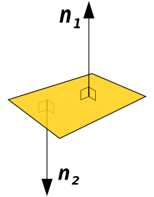
A polygon and two of its normal vectors

A normal to a surface at a point is the same as a normal to the tangent plane to the same surface at the same point.

In geometry, a normal is an object such as a line or vector that is perpendicular to a given object. For example, in two dimensions, the normal line to a curve at a given point is the line perpendicular to the tangent line to the curve at the point.

In three dimensions, a surface normal, or simply normal, to a surface at a point P is a vector that is perpendicular to the tangent plane to that surface at P. The word "normal" is also used as an adjective: a line normal to a plane, the normal component of a force, the normal vector, etc. The concept of normality generalizes to orthogonality.

The concept has been generalized to differentiable manifolds of arbitrary dimension embedded in a Euclidean space. The normal vector space or normal space of a manifold at a point P is the set of the vectors which are orthogonal to the tangent space at P. In the case of differential curves, the curvature vector is a normal vector of special interest.

The normal is often used in computer graphics to determine a surface's orientation toward a light source for flat shading, or the orientation of each of the corners (vertices) to mimic a curved surface with Phong shading.

Normal to surfaces in 3D space

Calculating a surface normal

For a convex polygon (such as a triangle), a surface normal can be calculated as the vector cross product of two (non-parallel) edges of the polygon.

For a plane given by the equation ax+by+cz+d=0displaystyle ax+by+cz+d=0, the vector (a,b,c)displaystyle (a,b,c) is a normal.

For a plane whose equation is given in parametric form

r(α,β)=a+αb+βcdisplaystyle mathbf r (alpha ,beta )=mathbf a +alpha mathbf b +beta mathbf c ,

i.e., a is a point on the plane and b and c are (non-parallel) vectors lying on the plane, the normal to the plane is a vector normal to both b and c which can be found as the cross product b×cdisplaystyle mathbf b times mathbf c .

For a hyperplane in n + 1 dimensions, again given by its parametric representation

r=a0+α1a1+⋯+αnandisplaystyle mathbf r =mathbf a _0+alpha _1mathbf a _1+cdots +alpha _nmathbf a _n,

where a₀ is a point on the hyperplane and a_i for i = 1, ..., n are non-parallel vectors lying on the hyperplane, a normal to the hyperplane is any vector in the null space of A where A is given by

A=[a1…an]displaystyle A=[mathbf a _1dots mathbf a _n].

That is, any vector orthogonal to all in-plane vectors is by definition a surface normal.

If a (possibly non-flat) surface S is parameterized by a system of curvilinear coordinates x(s, t), with s and t real variables, then a normal is given by the cross product of the partial derivatives

∂x∂s×∂x∂t.displaystyle partial mathbf x over partial stimes partial mathbf x over partial t.

If a surface S is given implicitly as the set of points (x,y,z)displaystyle (x,y,z) satisfying F(x,y,z)=0displaystyle F(x,y,z)=0, then, a normal at a point (x,y,z)displaystyle (x,y,z) on the surface is given by the gradient

∇F(x,y,z).displaystyle nabla F(x,y,z).

since the gradient at any point is perpendicular to the level set, and F(x,y,z)=0displaystyle F(x,y,z)=0 (the surface) is a level set of Fdisplaystyle F.

For a surface S given explicitly as a function f(x,y)displaystyle f(x,y) of the independent variables x,ydisplaystyle x,y (e.g., f(x,y)=a00+a01y+a10x+a11xydisplaystyle f(x,y)=a_00+a_01y+a_10x+a_11xy), its normal can be found in at least two equivalent ways.
The first one is obtaining its implicit form F(x,y,z)=z−f(x,y)=0displaystyle F(x,y,z)=z-f(x,y)=0, from which the normal follows readily as the gradient

∇F(x,y,z)displaystyle nabla F(x,y,z).

(Notice that the implicit form could be defined alternatively as

F(x,y,z)=f(x,y)−zdisplaystyle F(x,y,z)=f(x,y)-z;

these two forms correspond to the interpretation of the surface being oriented upwards or downwards, respectively, as a consequence of the difference in the sign of the partial derivative ∂F/∂zdisplaystyle partial F/partial z.)
The second way of obtaining the normal follows directly from the gradient of the explicit form,

∇f(x,y)displaystyle nabla f(x,y);

by inspection,

∇F(x,y,z)=k^−∇f(x,y)displaystyle nabla F(x,y,z)=hat mathbf k -nabla f(x,y), where k^displaystyle hat mathbf k is the upward unit vector.

This is equal to ∇F(x,y,z)=k^−∂f(x,y)∂xi^−∂f(x,y)∂yj^displaystyle nabla F(x,y,z)=hat mathbf k -frac partial f(x,y)partial xhat mathbf i -frac partial f(x,y)partial yhat mathbf j , where i^displaystyle hat mathbf i and j^displaystyle hat mathbf j are the x and y unit vectors.

If a surface does not have a tangent plane at a point, it does not have a normal at that point either. For example, a cone does not have a normal at its tip nor does it have a normal along the edge of its base. However, the normal to the cone is defined almost everywhere. In general, it is possible to define a normal almost everywhere for a surface that is Lipschitz continuous.

Uniqueness of the normal

A vector field of normals to a surface

A normal to a surface does not have a unique direction; the vector pointing in the opposite direction of a surface normal is also a surface normal. For a surface which is the topological boundary of a set in three dimensions, one can distinguish between the inward-pointing normal and outer-pointing normal, which can help define the normal in a unique way. For an oriented surface, the surface normal is usually determined by the right-hand rule. If the normal is constructed as the cross product of tangent vectors (as described in the text above), it is a pseudovector.

Transforming normals

Note: in this section we only use the upper 3x3 matrix, as translation is irrelevant to the calculation

When applying a transform to a surface it is often useful to derive normals for the resulting surface from the original normals.

Specifically, given a 3x3 transformation matrix M, we can determine the matrix W that transforms a vector n perpendicular to the tangent plane t into a vector n′ perpendicular to the transformed tangent plane M t, by the following logic:

Write n′ as W n. We must find W.

W n perpendicular to M t

⟺(Wn)⋅(Mt)=0displaystyle iff (Wn)cdot (Mt)=0

⟺(Wn)T(Mt)=0displaystyle iff (Wn)^T(Mt)=0

⟺(nTWT)(Mt)=0displaystyle iff (n^TW^T)(Mt)=0

⟺nT(WTM)t=0displaystyle iff n^T(W^TM)t=0

Clearly choosing W such that WTM=Idisplaystyle W^TM=I, or W=M−1Tdisplaystyle W=M^-1^T will satisfy the above equation, giving a Wndisplaystyle Wn perpendicular to Mtdisplaystyle Mt, or an n′ perpendicular to t′, as required.

Therefore, one should use the inverse transpose of the linear transformation when transforming surface normals. The inverse transpose is equal to the original matrix if the matrix is orthonormal, i.e. purely rotational with no scaling or shearing.

Hypersurfaces in n-dimensional space

The definition of a normal to a surface in three-dimensional space can be extended to (n−1)displaystyle (n-1)-dimensional hypersurfaces in a n-dimensional space. A hypersurface may be locally defined implicitly as the set of points (x1,x2,…,xn)displaystyle (x_1,x_2,ldots ,x_n) satisfying an equation F(x1,x2,…,xn)=0displaystyle F(x_1,x_2,ldots ,x_n)=0, where Fdisplaystyle F is a given scalar function. If Fdisplaystyle F is continuously differentiable then the hypersurface is a differentiable manifold in the neighbourhood of the points where the gradient is not null. At these points the normal vector space has dimension one and is generated by the gradient

∇F(x1,x2,…,xn)=(∂F∂x1,∂F∂x2,…,∂F∂xn).displaystyle nabla F(x_1,x_2,ldots ,x_n)=left(tfrac partial Fpartial x_1,tfrac partial Fpartial x_2,ldots ,tfrac partial Fpartial x_nright),.

The normal line at a point of the hypersurface is defined only if the gradient is not null. It is the line passing through the point and having the gradient as direction.

Varieties defined by implicit equations in n-dimensional space

A differential variety defined by implicit equations in the n-dimensional space is the set of the common zeros of a finite set of differential functions in n variables

f1(x1,…,xn),…,fk(x1,…,xn).displaystyle f_1(x_1,ldots ,x_n),ldots ,f_k(x_1,ldots ,x_n).

The Jacobian matrix of the variety is the k×n matrix whose i-th row is the gradient of f_i. By implicit function theorem, the variety is a manifold in the neighborhood of a point of it where the Jacobian matrix has rank k. At such a point P, the normal vector space is the vector space generated by the values at P of the gradient vectors of the f_i.

In other words, a variety is defined as the intersection of k hypersurfaces, and the normal vector space at a point is the vector space generated by the normal vectors of the hypersurfaces at the point.

The normal (affine) space at a point P of the variety is the affine subspace passing through P and generated by the normal vector space at P.

These definitions may be extended verbatim to the points where the variety is not a manifold.

Example

Let V be the variety defined in the 3-dimensional space by the equations

xy=0,z=0.displaystyle x,y=0,quad z=0,.

This variety is the union of the x-axis and the y-axis.

At a point (a, 0, 0), where a ≠ 0, the rows of the Jacobian matrix are (0, 0, 1) and (0, a, 0). Thus the normal affine space is the plane of equation x = a. Similarly, if b ≠ 0, the normal plane at (0, b, 0) is the plane of equation y = b.

At the point (0, 0, 0) the rows of the Jacobian matrix are (0, 0, 1) and (0, 0, 0). Thus the normal vector space and the normal affine space have dimension 1 and the normal affine space is the z-axis.

Uses

• Surface normals are essential in defining surface integrals of vector fields.


• Surface normals are commonly used in 3D computer graphics for lighting calculations; see Lambert's cosine law.


• Surface normals are often adjusted in 3D computer graphics by normal mapping.


• 
  Render layers containing surface normal information may be used in Digital compositing to change the apparent lighting of rendered elements.

Normal in geometric optics

Diagram of specular reflection

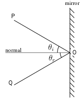
The normal is the line perpendicular to the surface of an optical medium at a given point.^[1] In reflection of light, the angle of incidence and the angle of reflection are respectively the angle between the normal and the incident ray (on the plane of incidence) and the angle between the normal and the reflected ray.

See also

• Ellipsoid normal vector


• Pseudovector


• Dual space


• Vertex normal

References

External links

• Weisstein, Eric W. "Normal Vector". MathWorld.


• An explanation of normal vectors from Microsoft's MSDN


• Clear pseudocode for calculating a surface normal from either a triangle or polygon.

References

^ "The Law of Reflection". The Physics Classroom Tutorial. Retrieved 2008-03-31..mw-parser-output cite.citationfont-style:inherit.mw-parser-output .citation qquotes:"""""""'""'".mw-parser-output .citation .cs1-lock-free abackground:url("//upload.wikimedia.org/wikipedia/commons/thumb/6/65/Lock-green.svg/9px-Lock-green.svg.png")no-repeat;background-position:right .1em center.mw-parser-output .citation .cs1-lock-limited a,.mw-parser-output .citation .cs1-lock-registration abackground:url("//upload.wikimedia.org/wikipedia/commons/thumb/d/d6/Lock-gray-alt-2.svg/9px-Lock-gray-alt-2.svg.png")no-repeat;background-position:right .1em center.mw-parser-output .citation .cs1-lock-subscription abackground:url("//upload.wikimedia.org/wikipedia/commons/thumb/a/aa/Lock-red-alt-2.svg/9px-Lock-red-alt-2.svg.png")no-repeat;background-position:right .1em center.mw-parser-output .cs1-subscription,.mw-parser-output .cs1-registrationcolor:#555.mw-parser-output .cs1-subscription span,.mw-parser-output .cs1-registration spanborder-bottom:1px dotted;cursor:help.mw-parser-output .cs1-ws-icon abackground:url("//upload.wikimedia.org/wikipedia/commons/thumb/4/4c/Wikisource-logo.svg/12px-Wikisource-logo.svg.png")no-repeat;background-position:right .1em center.mw-parser-output code.cs1-codecolor:inherit;background:inherit;border:inherit;padding:inherit.mw-parser-output .cs1-hidden-errordisplay:none;font-size:100%.mw-parser-output .cs1-visible-errorfont-size:100%.mw-parser-output .cs1-maintdisplay:none;color:#33aa33;margin-left:0.3em.mw-parser-output .cs1-subscription,.mw-parser-output .cs1-registration,.mw-parser-output .cs1-formatfont-size:95%.mw-parser-output .cs1-kern-left,.mw-parser-output .cs1-kern-wl-leftpadding-left:0.2em.mw-parser-output .cs1-kern-right,.mw-parser-output .cs1-kern-wl-rightpadding-right:0.2em